Hey there, nice to see you back for this fourth and final part of our DevOps tutorial series! 😃

Today’s tutorial will be mainly divided into two parts. First we’ll finalised our cloud data architecture and make sure that it updates itself automatically on a daily basis. Then, in a second time we’ll hop onto the creation of our Grafana dashboard and see how we can connect our ethdb database to a Grafana instance in order to create our ETH analytics dashboard.

Part 1: Cloud data architecture finalization

Alright so first thing first, now that we have at our disposal our basic cloud data architecture with each of our tables initialised we need to create python scripts enabling us to update each of those with new daily metrics.

Observation: In the case of the daily_metrics and delayed_metrics tables given that we only extracted the latest daily metric value available we don’t need to recreate additional python scripts and can directly used the python functions that we used in our table_init2 and table_init3 python scripts.

Alright so let’s focus on the case of the historical_metrics and network_growth tables. So here basically the idea, is to create a python script in order to add on a daily basis the new daily metrics value to each tables.

Starting, with our historical_metrics table, let’s create a new updating python scripts called historical_daily.py in our code folder using the following command:

$ nano historical_daily.py

From there copy and paste the code that you can find here in the corresponding file in Github.

Observation: Here the code is basically exactly the same that we used before in our previous tutorial in our table_init.py script at the difference that here we’re only focusing on extracting the metric value for the current day.

Alright from there using the same process let’s take care of our network_growth table. So first we’ll create a new python script using the following command:

$ nano network_growth.py

From there copy and paste the content of the github file of the same name:

Alright, now we have to make those scripts executable and run them. To do so we’ll use the following commands presented in our previous tutorial:

$ chmod +x historical_daily.py 
$ chmod +x network_growth.py 
$ ./historical_daily.py 
$ ./network_growth.py

Here if everything goes well you should be met with our usual prompt message '“Process done'“ after the running of each of our python scripts.

Note: if you want to double check, feel free to use the same process explained in our previous tutorial using the Postgres user and your local instance of psql.

Alright so now that we’re all set and have our full data architecture, let’s automate this daily updating process. To do so, first we’ll need to create a python script that we’ll call main.py which will call all the functions we need to perform a full daily update of all our tables composing our cloud data architecture.

So first let’s create, that new python script in our code folder using the following command:

$ nano main.py

From there as usual copy the content of the corresponding github file in your editor:

As you can see here, this file is pretty straightforward we basically just import each functions that we need from their respective python scripts and run them one after another.

Alright so from there, as always we need to make this script executable using the following command:

$ chmod +x main.py

Once it’s done the last thing we need to do, is to ask our cloud server ro automatically run on a daily basis this script. To do so, we’ll use a linux tool called crontab enabling us to ask the computer to perform a set of task on a periodical basis. So first let’s open crontab using the following command:

$ crontab -e

Choose the easiest editor by typing 1:

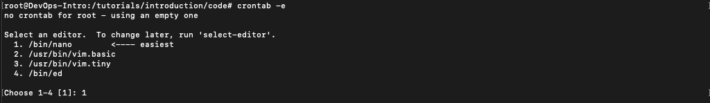
Normally you should be met with the following editor:

From there type the following command below the comments, save and exit the editor.

$ 0 9 * * * ./main.py

See here for crontab time converter

And that’s it we finally have a complete full cloud data architecture querying and storing our needed metrics value on a daily basis 👍

Alright so that’s a pretty big part done, so don’t hesitate to make a quick coffee break here if you need it before heading to the second part ☕

Part 2 Grafana dashboard creation

Alright so let’s start building our Grafana dashboard. First, if you haven’t already created one go on the Grafana website and follow the onboarding steps in order to create an account.

Once you’re done you should be able to see the following screen:

So first, let’s create our dashboard. To do so, hoover over the dashboard icon and click on “new dashboard”.

From there click on '“Add new panel” and click on “save” in order to save your new dashboard as shown below:

Alright, so now let’s connect our ethdb database stored in our cloud server to our Grafana instance in order to get access to our ethereum network metrics.

So first let’s click on configuration and go into Data sources.

Once you’re there click on add datasource

From there seach for postgreSQL and select it in order to add a new PostgreSQL data source to your Grafana instance.

Here we have to specify the following connection parameters:

• Name -- the Grafana name we want to give to our data source. Here we’ll call it ethdb

• Host -- which corresponds to the IP address of our DO server and the port that Grafana should use to connect to it here it is “:5432” (as per Digital Ocean default parameters)

• User -- which corresponds to the user that we use to connect to our database located in our cloud server. Here we’ll use our previously created user called “myuser” the password being the password you assigned to your psql user.

• TLS/SSL Mode -- Disable

Once you specified all the parameters presented above, click on “Save & Test” and if everything goes smoothly you should see appear the following message

Alright so now that we connected successfully our ethdb database to our grafana instance let’s start building our Grafana dashboard. So first let’s get back to our dashboard and edit our panel

There click on data source and select ethdb

Once it’s done, in the query section click on the code option in order to be able to start writing SQL queries and use the following command:

select date, historical_prices 
from historical_metrics
order by date asc;

Upon running the query you should end up with the following result:

Don’t forget to select the “last 6 months” time range given that it is not the by default used time range by Grafana.

From there you can customize your graph as you want using the panel options and once you’re done don’t forget to save all your changes.

Alright so now that we’re down with our price chart let’s go ahead and create another panel in order to create our current price counter.

From there as before choose ethdb but this time copy and paste the following sql command in order to extract the current ETH price from our daily_metrics table.

select date, price 
from daily_metrics 
order by date desc
limit 1
;

Normally you should end up with the following result:

Here, switch the visualization from time series to stats and delete the threshold in the panel options before saving it.

Alright so now moving on to our daily volume counter using the same process and the following SQL command we obtain a counter with our daily volume.

select date, volume 
from daily_metrics
order by date desc
limit 1; 

Observation: Our volume here is expressed in billions so if you want to also show that in Grafana you can use a transformation by clicking on transformation and on the “Add field from calculation” button as shown below:

Then in order to only get your value in billion showed in the counter go to the panel options and select your newly added columns in the Fields section.

Alright so for the two other counters we’ll basically use the same process and use the following SQL queries.

Social Volume:

select date, socialvolume
from delayed_metrics
order by date desc
limit 1
;

24h active addresses:

select date, activeaddress 
from daily_metrics
order by date desc
limit 1;

Normally if everything goes right you should end up with a dashboard similar to the one below:

From there, the building steps being mostly the same in order to create the rest of the below dashboard I’ll let you try to do it on your own as an exercise by relying on the below code snippets showing you which sql queries you should use to create each of the neeeded dashboard components.

SQL queries:

Velocity

select date, volatility
from delayed_metrics
order by date desc
limit 1;

Marketcap

select date, historical_marketcap 
from historical_metrics
order by date asc
; 

Top holders

select date, topholders
from delayed_metrics
order by date desc 
limit 1; 

Github activity

select date, githubactivity
from delayed_metrics
order by date desc
limit 1; 

Dev Activity

select date, devactivity 
from delayed_metrics
order by date desc
limit 1;

Network Growth

select * 
from network_growth
order by date asc;

And that’s it !! 🥳🥳

So congrats if you reach the end of this tutorial serie, you’re now well equipped to go further and start tackling further challenges so be proud of yourself and as always don’t hesitate to play around with the code and fine-tune it to your liking 😃

In the future we’ll go further and introduce other DevOps notions such as kubernetes, docker and others tools so stay tuned if you’re interested to learn more about those and in the meantime have fun with all this new knowledge.

Take care 🖖