
Here is what we are going to cover:
- Forecasting Curve TVL.
- Curve TVL <> Defi TVL Correlation.
- Defi TVL <> BTC price Correlation.
- BTC Forecasting Model.
- Forecasting Curve Trading Volume.
- $CRV emission schedule
- Speculating on the revenue stream distribution for the TVL under Curve finance.
This article goes in-depth in constructing correlations with the past data to predict the future data to further analyze them.
With the future possible forecasts for Curve TVL, trading volume, and $CRV emissions, we could compute the required price increase in $CRV to generate a constant return on the TVL.
If this simple reading layout doesn’t excite you, you could scroll down to consume the same content as if it were a magazine. It might take a bit to load the magazine pages, your patience is well appreciated.
⚠ Disclaimer: There are risks associated with investing in virtual assets. The content is for informational purposes only, you should not construe any such information as investment or financial advice. You are responsible for evaluating the merits and risks associated with the use of any such information associated with DiligentDeer before making any financial decision. I won’t be responsible for any kind of financial profits or losses derived from your decisions. Financial and investment advice
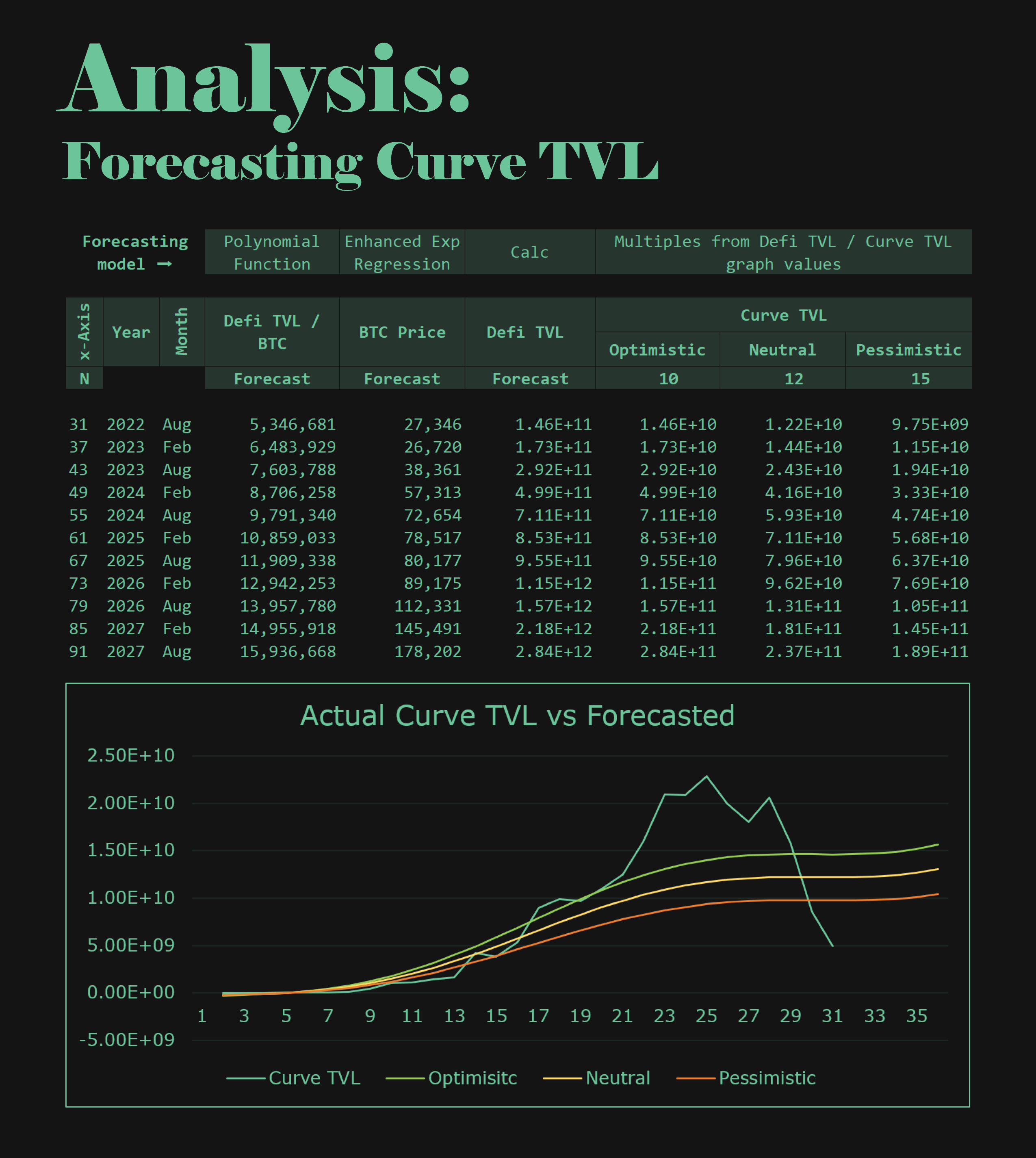
🧠Analysis: Forecasting Curve TVL
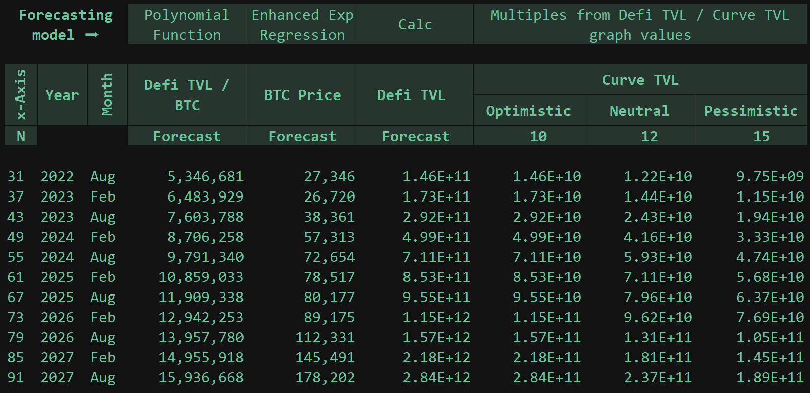
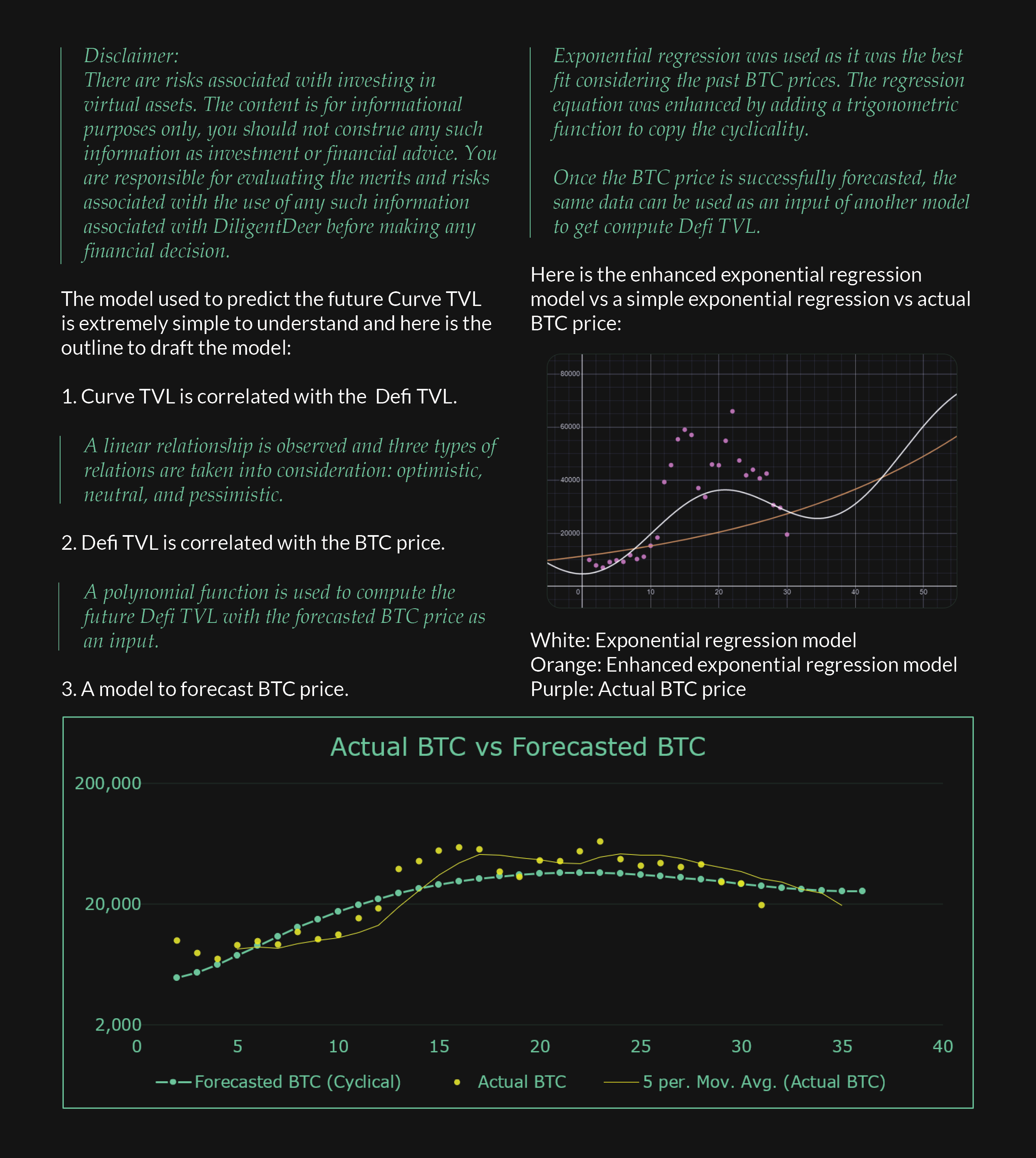
The model used to predict the future Curve TVL is extremely simple to understand and here is the outline to draft the model:
- Curve TVL is correlated with the Defi TVL.
A linear relationship is observed and three types of relations are taken into consideration: optimistic, neutral, and pessimistic.
- Defi TVL is correlated with the BTC price.
A polynomial function is used to compute the future Defi TVL with the forecasted BTC price as an input.
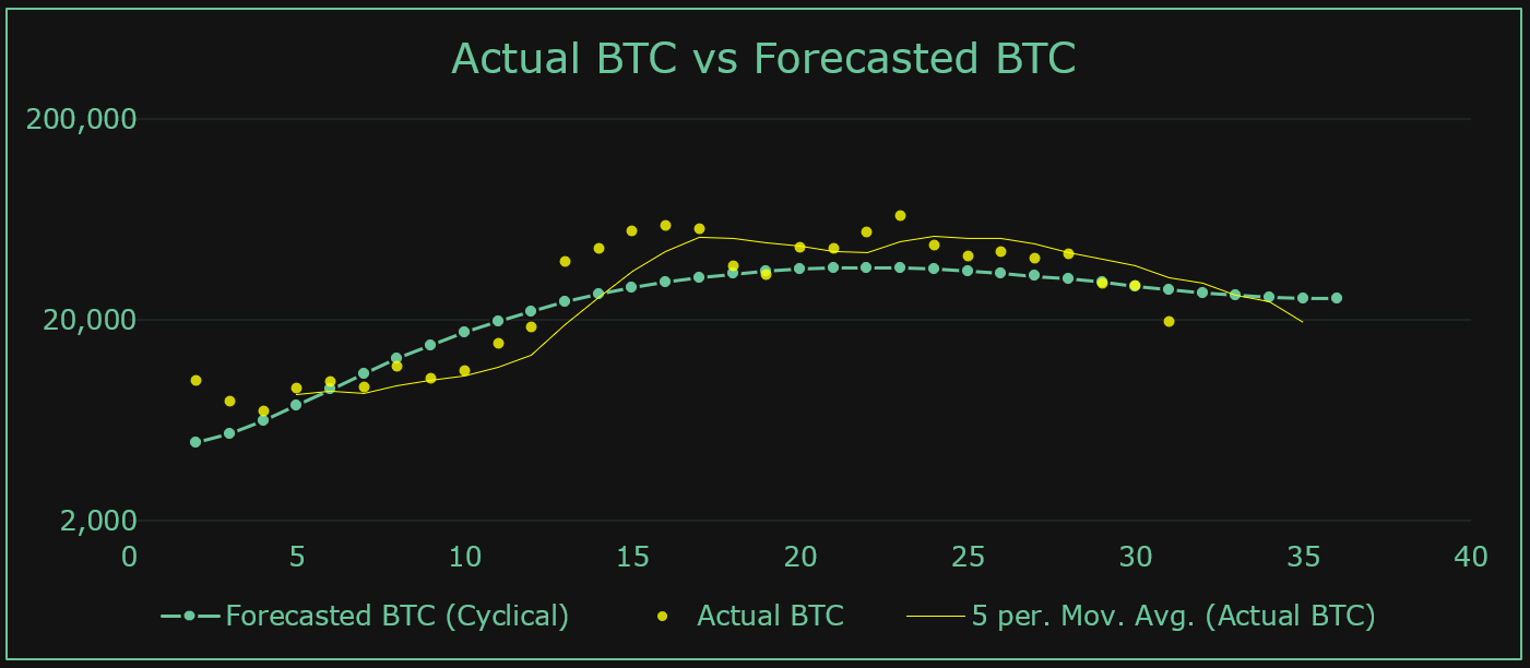
- A model to forecast BTC price
Exponential regression was used as it was the best fit considering the past BTC prices. The regression equation was enhanced by adding a trigonometric function to copy the cyclicality.
Once the BTC price is successfully forecasted, the same data can be used as an input of another model to get compute Defi TVL.
Enhanced exponential regression model vs a simple exponential regression vs actual BTC price:
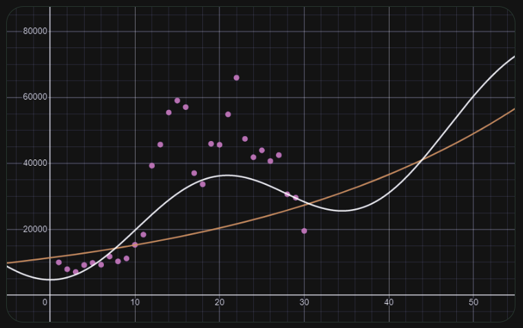
White: Exponential regression model
Orange: Enhanced exponential regression model
Purple: Actual BTC price
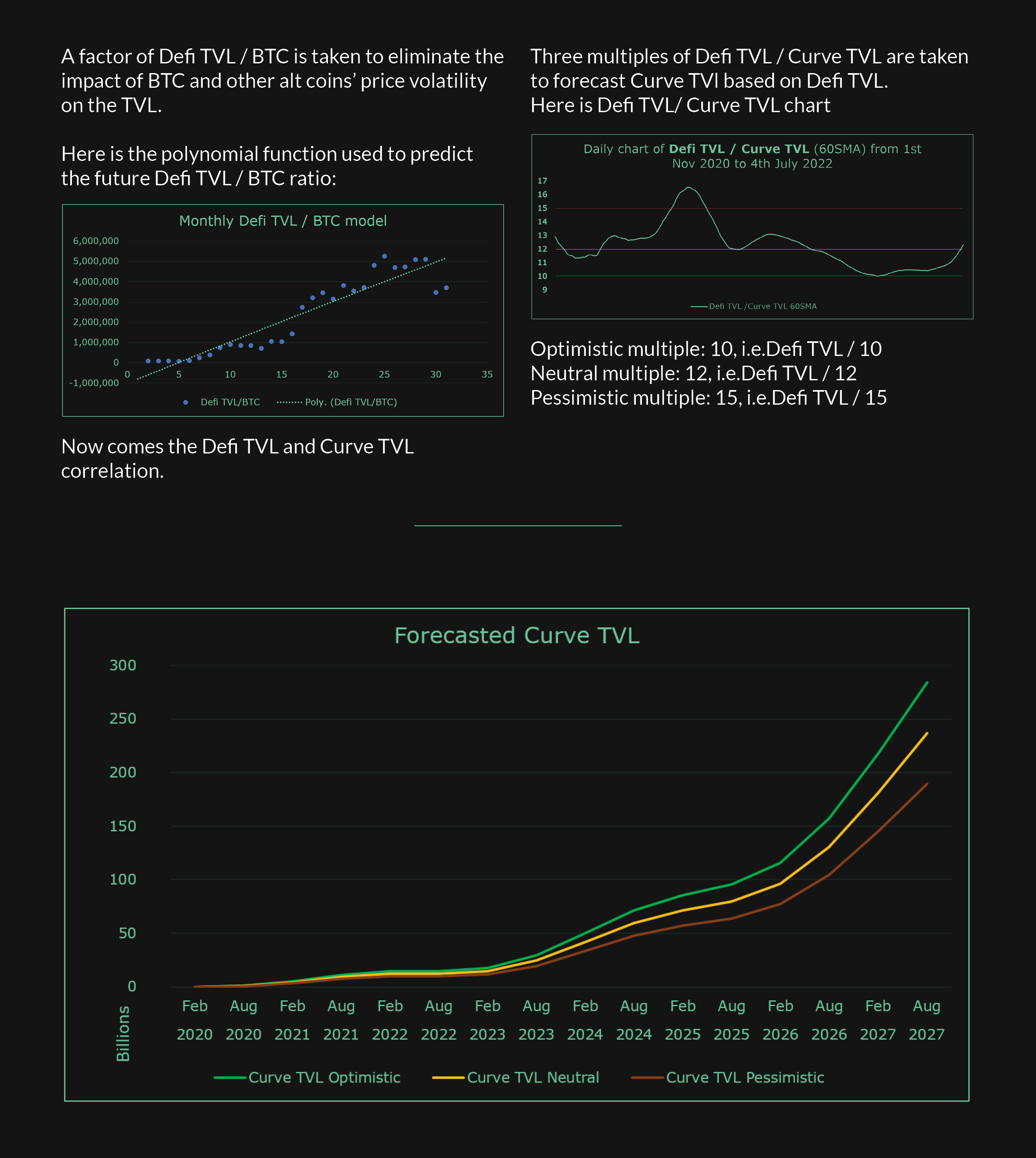
A factor of Defi TVL / BTC is taken to eliminate the impact of BTC and other alt coins’ price volatility on the TVL.
Polynomial function used to predict the future Defi TVL / BTC ratio:
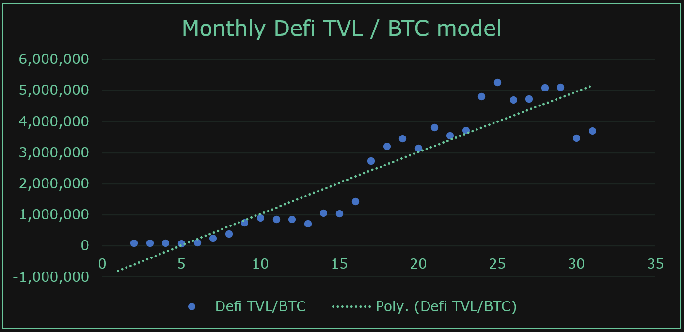
[PS: Defi TVL / BTC model takes into consideration the TVL growth due to the price impact of volatile assets through considering BTC price volatility.]
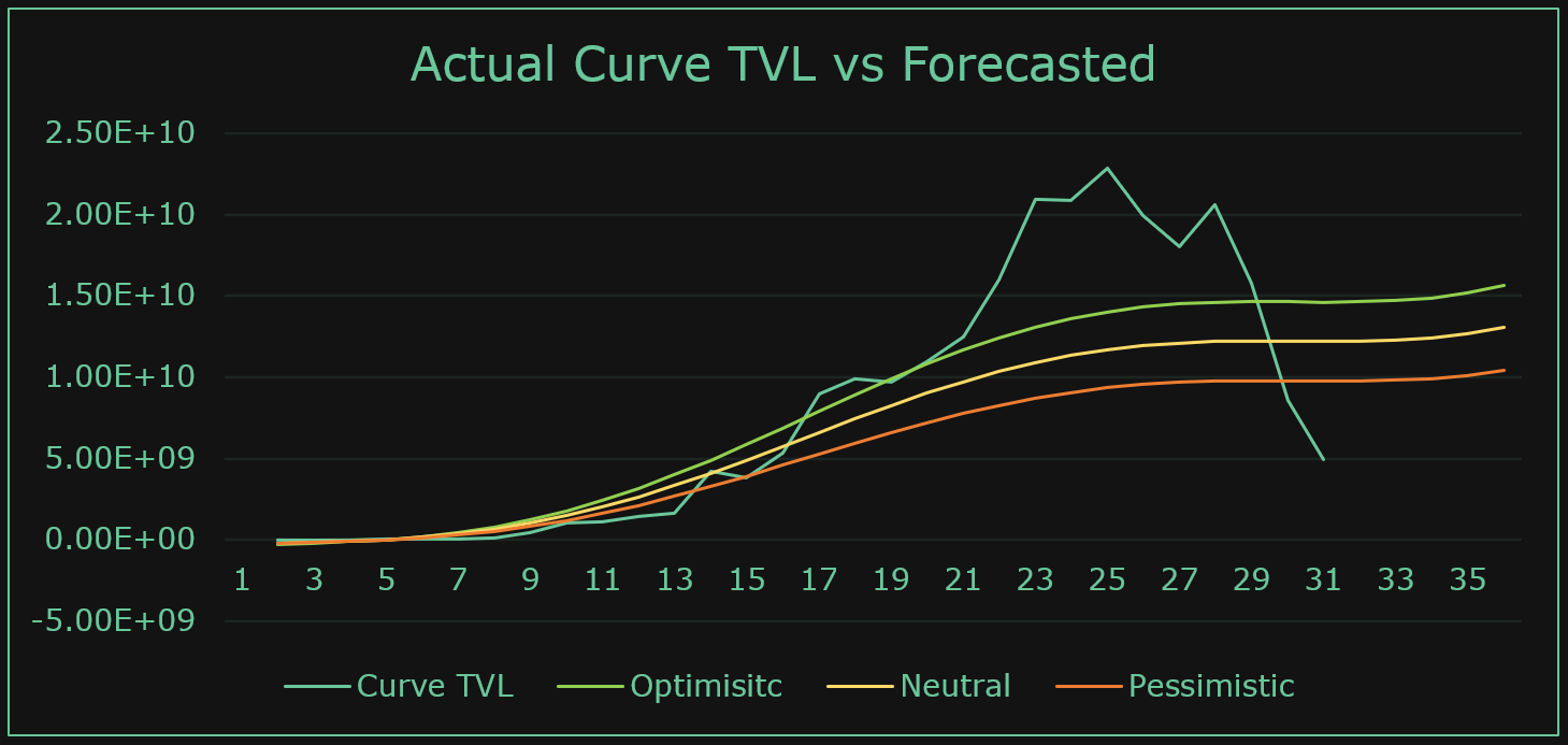
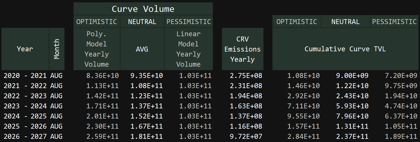
The Defi TVL and Curve TVL correlation.
Three multiples of Defi TVL / Curve TVL are taken to forecast Curve TVl based on Defi TVL.
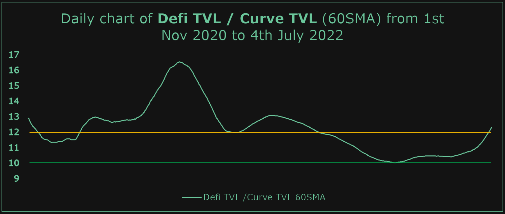
Optimistic multiple: 10, i.e.Defi TVL / 10
Neutral multiple: 12, i.e.Defi TVL / 12
Pessimistic multiple: 15, i.e.Defi TVL / 15
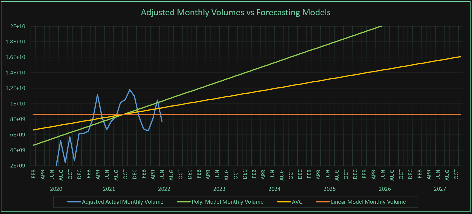
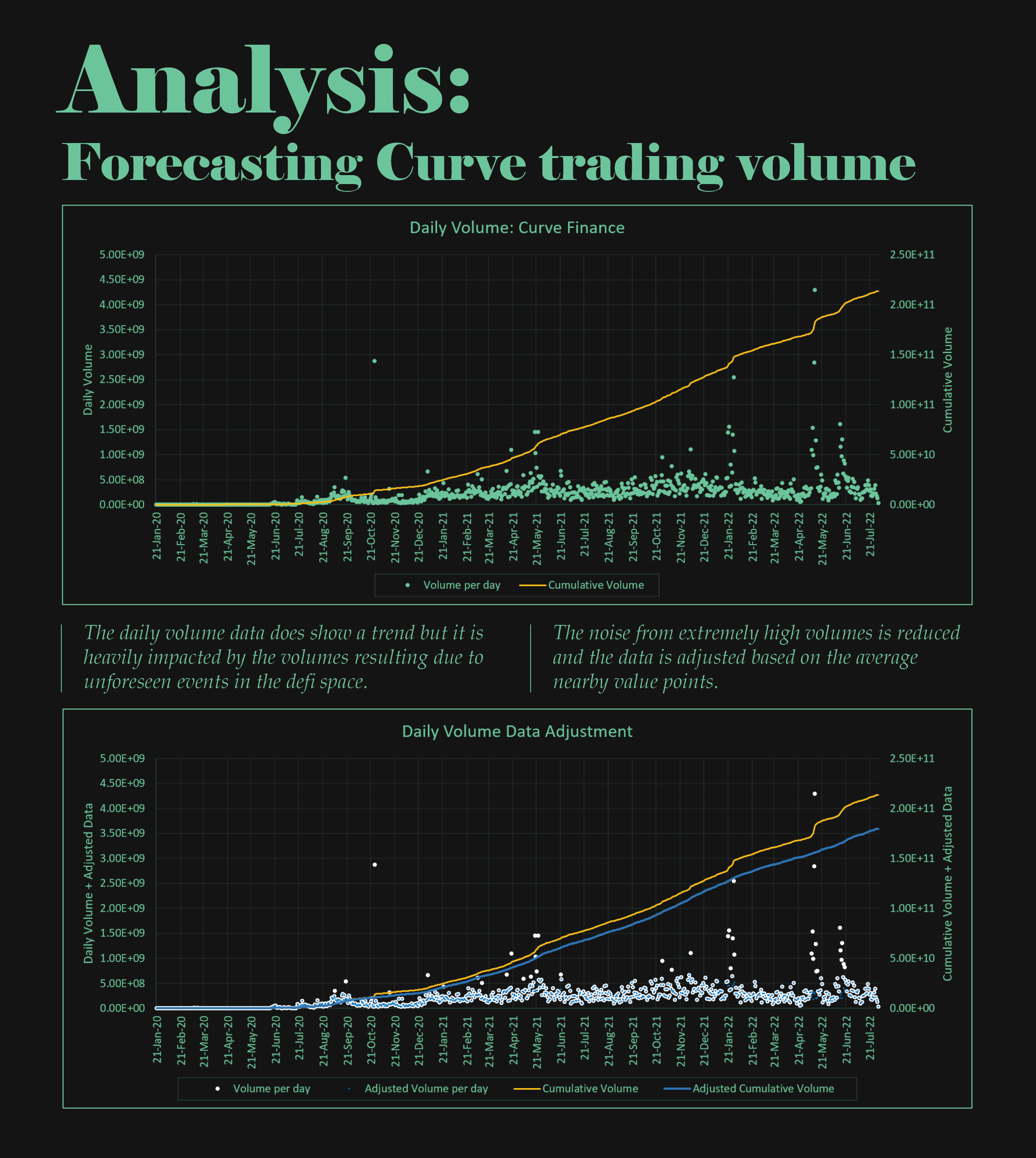
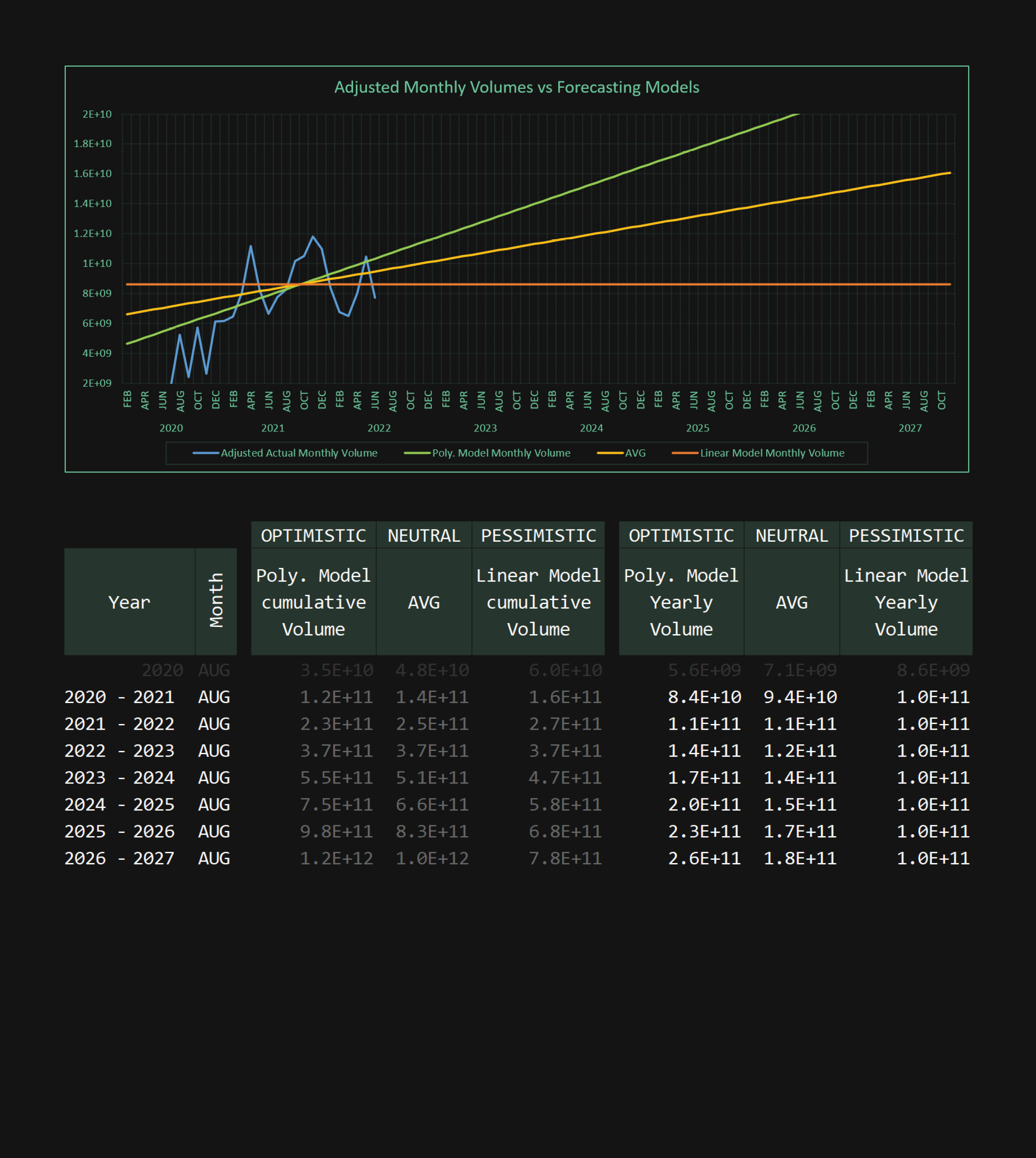
🧠Analysis: Forecasting Curve trading volume
The daily volume data does show a trend but it is heavily impacted by the volumes resulting due to unforeseen events in the defi space.
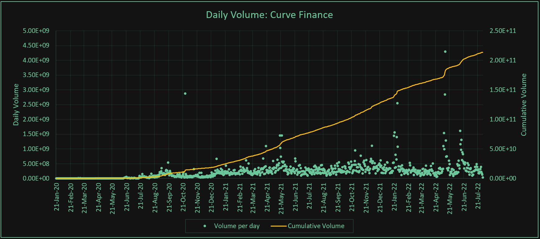
The noise from extremely high volumes is reduced and the data is adjusted based on the average nearby value points.
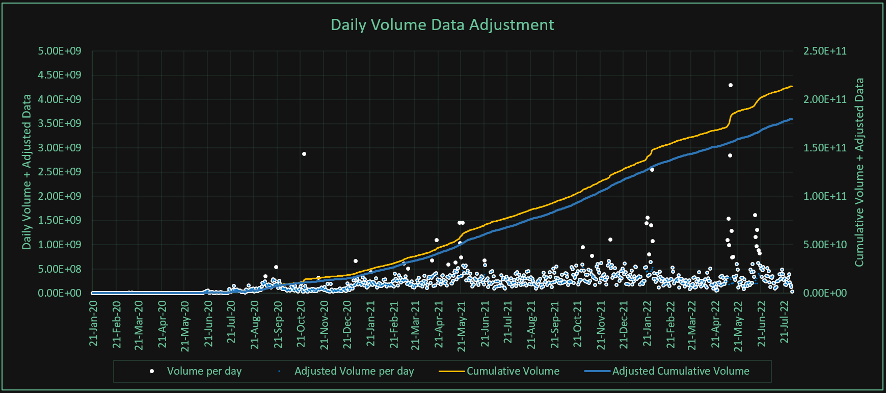
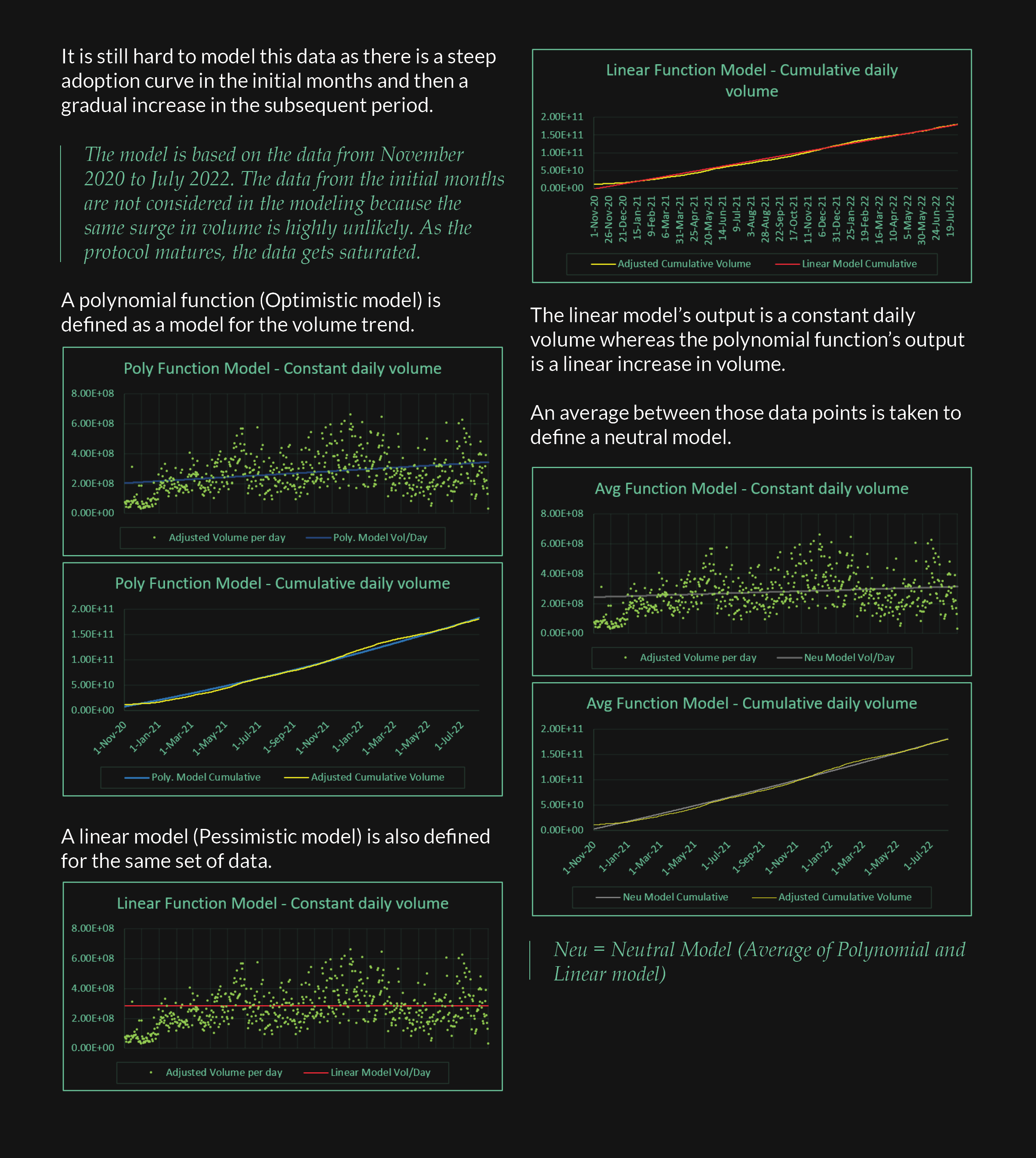
It is still hard to model this data as there is a steep adoption curve in the initial months and then a gradual increase in the subsequent period.
The model is based on the data from November 2020 to July 2022. The data from the initial months are not considered in the modeling because the same surge in volume is highly unlikely. As the protocol matures, the data gets saturated.
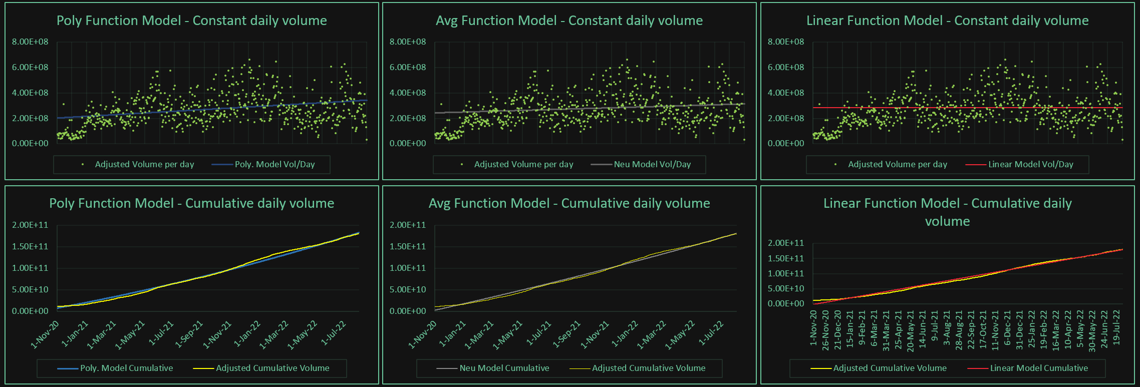
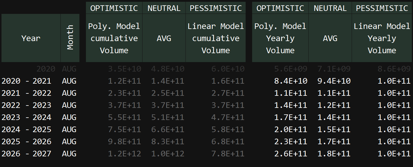
- A polynomial function (Optimistic model) is defined as a model for the volume trend.
- A linear model (Pessimistic model) is also defined for the same set of data.
- The linear model’s output is a constant daily volume whereas the polynomial function’s output is a linear increase in volume.
- An average between those data points is taken to define a neutral model. Neu = Neutral Model (Average of Polynomial and Linear model)
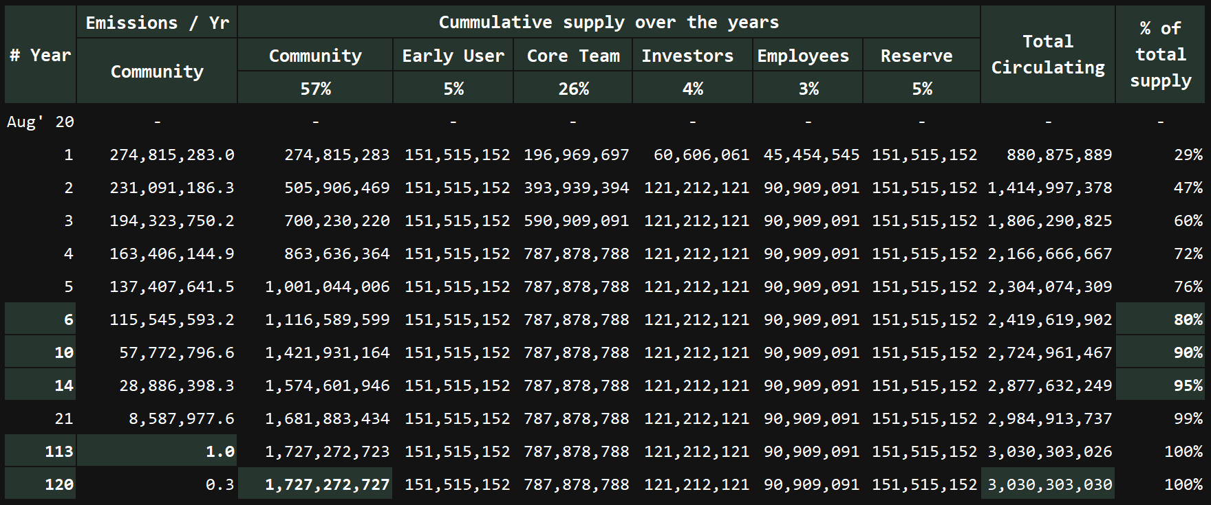
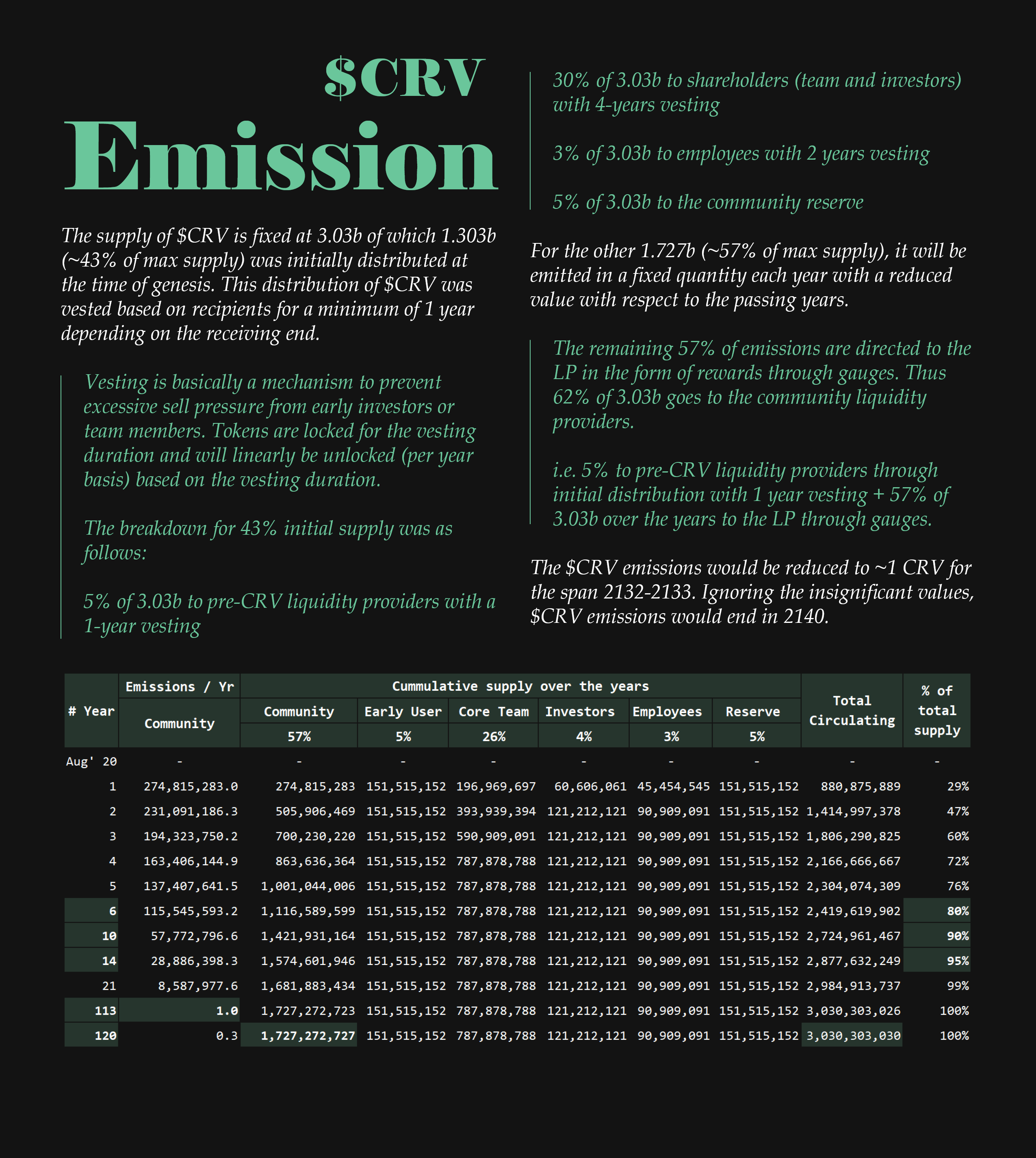
🧠$CRV Emissions
The supply of $CRV is fixed at 3.03b of which 1.303b (~43% of max supply) was initially distributed at the time of genesis. This distribution of $CRV was vested based on recipients for a minimum of 1 year depending on the receiving end.
Vesting is basically a mechanism to prevent excessive sell pressure from early investors or team members. Tokens are locked for the vesting duration and will linearly be unlocked (per year basis) based on the vesting duration.
The breakdown for 43% initial supply was as follows:
5% of 3.03b to pre-CRV liquidity providers with a 1-year vesting
30% of 3.03b to shareholders (team and investors) with 4-years vesting
3% of 3.03b to employees with 2 years vesting
5% of 3.03b to the community reserve
For the other 1.727b (~57% of max supply), it will be emitted in a fixed quantity each year with a reduced value with respect to the passing years.
The remaining 57% of emissions are directed to the LP in the form of rewards through gauges. Thus 62% of 3.03b goes to the community liquidity providers.
i.e. 5% to pre-CRV liquidity providers through initial distribution with 1 year vesting + 57% of 3.03b over the years to the LP through gauges.
The $CRV emissions would be reduced to ~1 CRV for the span 2132-2133. Ignoring the insignificant values, $CRV emissions would end in 2140.
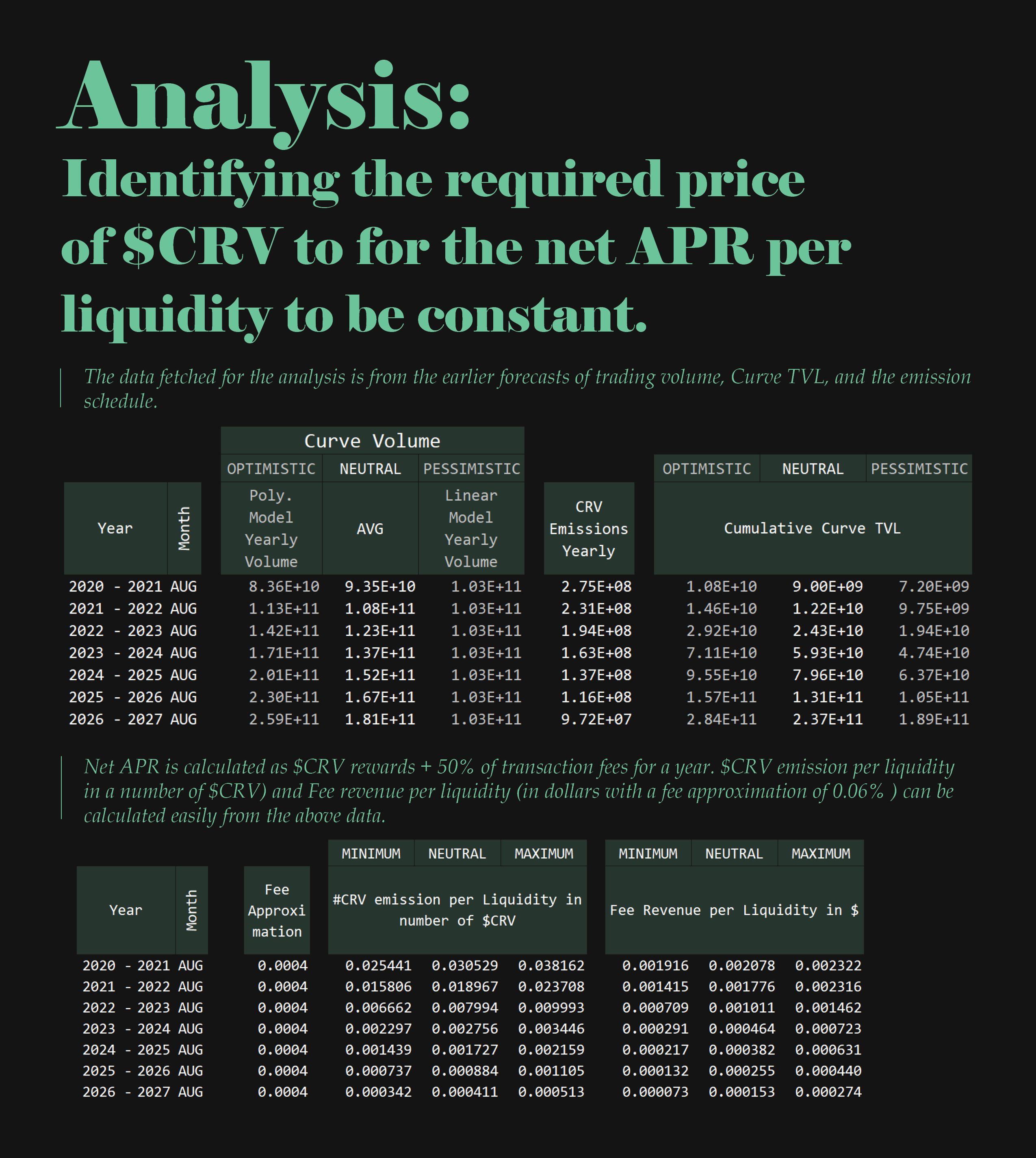
🧠Analysis: Identifying the required price of $CRV for the net APR per liquidity to be constant.
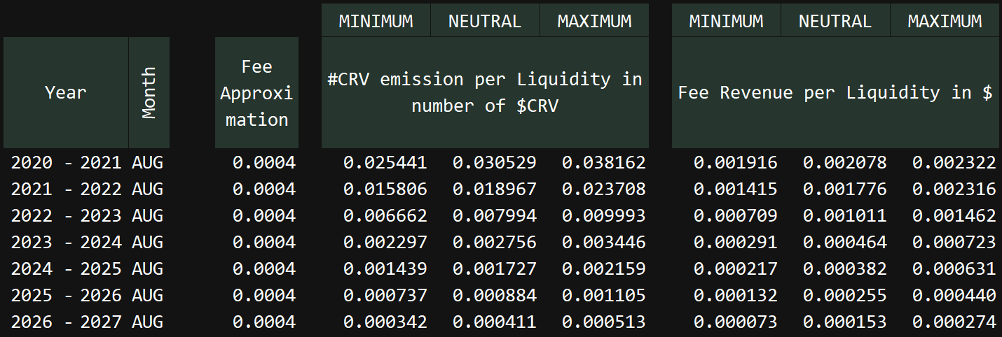
The data fetched for the analysis is from the earlier forecasts of trading volume, Curve TVL, and the emission schedule.
Net APR is calculated as $CRV rewards + 50% of transaction fees for a year. $CRV emission per liquidity in a number of $CRV) and Fee revenue per liquidity (in dollars with a fee approximation of 0.06% ) can be calculated easily from the above data.
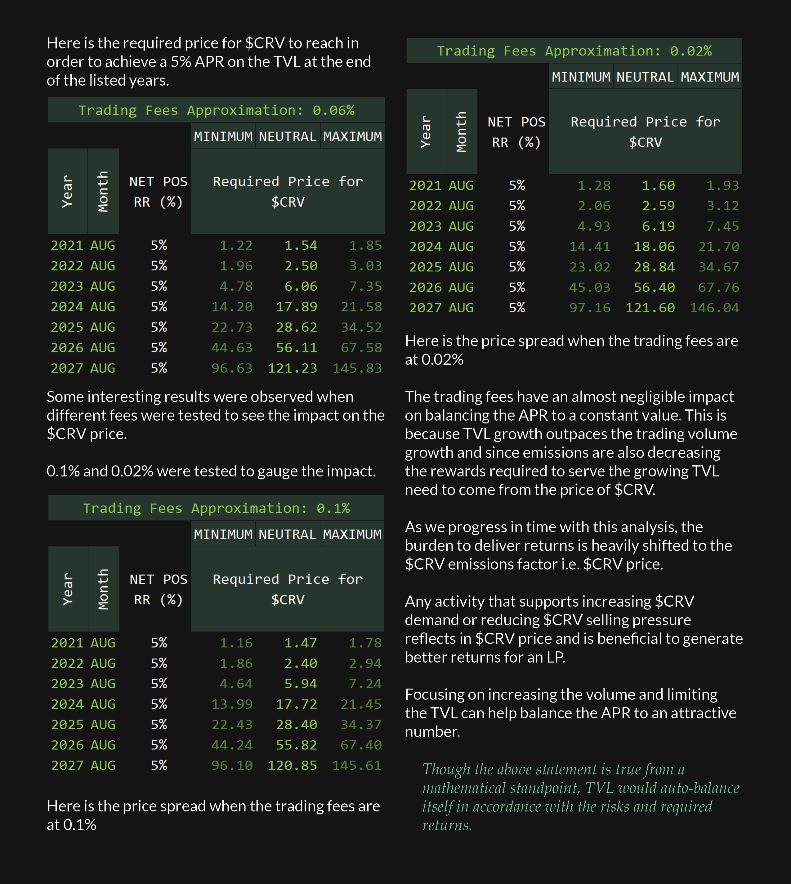
Here is the required price for $CRV to reach in order to achieve a 5% APR on the TVL at the end of the listed years.
Some interesting results were observed when different fees were tested to see the impact on the $CRV price.
0.1% and 0.02% were tested and compared with 0.06% fees to gauge the impact.
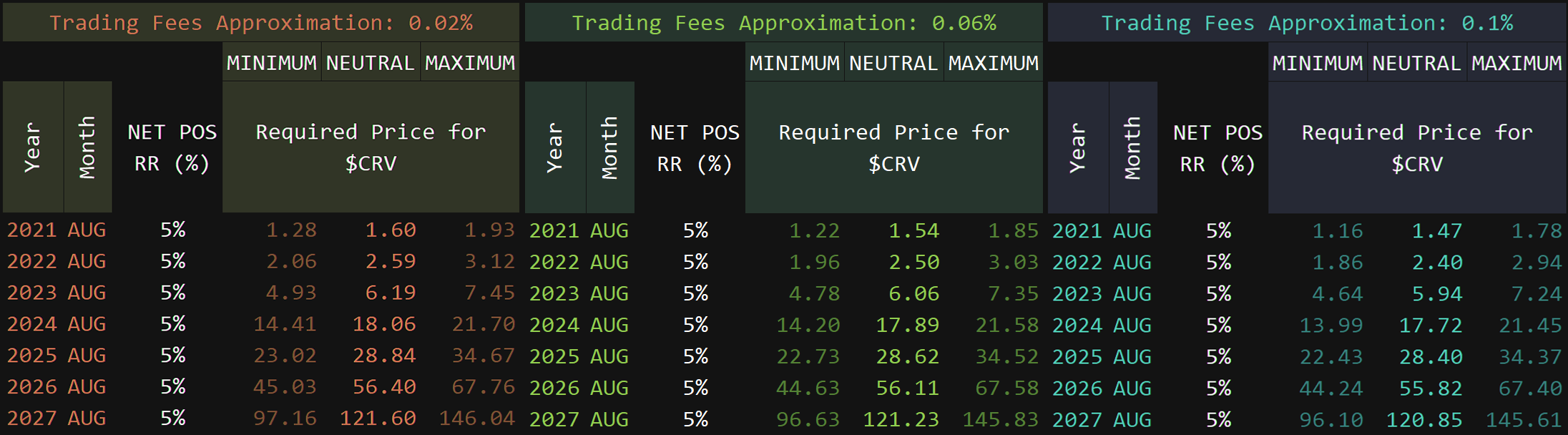
The trading fees have an almost negligible impact on balancing the APR to a constant value. This is because TVL growth outpaces the trading volume growth and since emissions are also decreasing the rewards required to serve the growing TVL need to come from the price of $CRV.
As we progress in time with this analysis, the burden to deliver returns is heavily shifted to the $CRV emissions factor i.e. $CRV price.
Any activity that supports increasing $CRV demand or reducing $CRV selling pressure reflects in $CRV price and is beneficial to generate better returns for an LP.
Focusing on increasing the volume and limiting the TVL can help balance the APR to an attractive number.
Though the above statement is true from a mathematical standpoint, TVL would auto-balance itself in accordance with the risks and required returns.
Thank you for being here.
You can provide the same value by sharing this article with your circle.
You could even contribute/support these articles by owning one ✌.
Thank you for being here.
You can provide the same value by sharing this article with your circle.
You could even contribute/support these articles by owning one ✌.