In my previous post, I conducted a fairly thorough walkthrough of the game of blackjack, reinforcement learning, Q learning, and various analyses. In this post, I’ll introduce the concept of Deep Reinforcement Learning (or, Deep Q Learning).

Why Deep Q Learning?

In traditional frameworks for Q Learning, we store state-action pairs and their associated Q value in memory. In the game of blackjack, this is a tractable solution, only if we exclude card count entirely. To review, let’s take an arbitrary state in blackjack as below:

(player_total, house_shows, useable_ace)

player_total can range from 4-21, house_shows can range from 2-11 (we’ll count Ace as 11), and useable_ace is a binary variable. For each of these, we have associated actions: Hit, Stay, Double, Split, Surrender (excluding insurance for now). For a computer, storing all these state-action pairs in memory is feasible, and can be accomplished as a simple dictionary in python.

However, what if we have more states, more actions, or what if some of the states are continuous values? The number of state-action pairs can grow drastically, to the point where storing all of these possibilities in memory is completely intractable. That’s where Deep Q Learning comes in.

What is Deep Q Learning?

In Deep Q Learning, rather than learning the Q function directly, we are able to learn an approximation for this Q function. Deep Neural Networks can theoretically learn any function, through a combination of linear and non-linear layers. The best depiction I’ve seen on Q Learning vs. Deep Q Learning is the following:

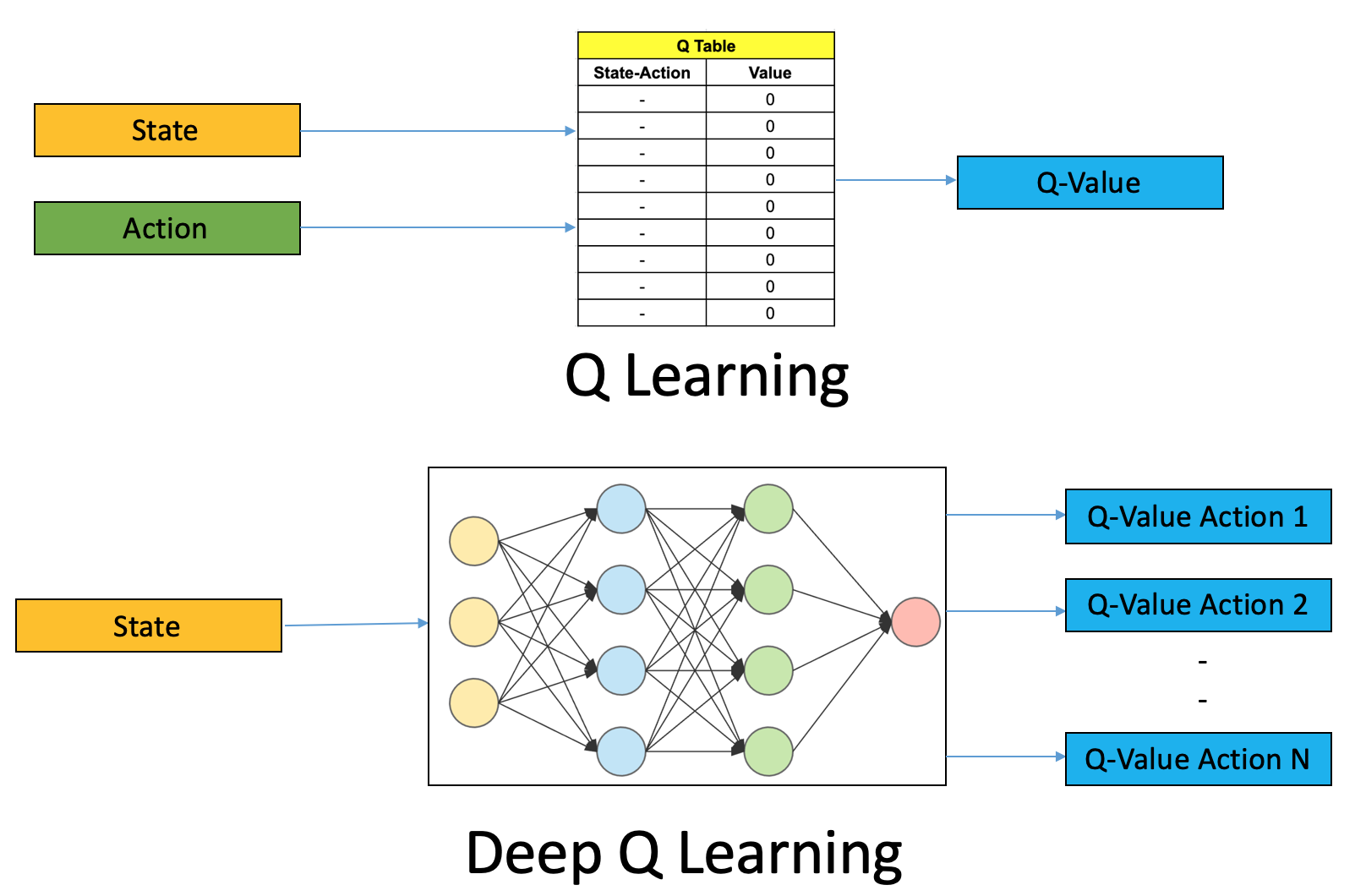
Consider Q learning as a look-up table. The input is the state-action pair as the key, and the resulting value is the Q value of interest for that action in the given state. In Deep Q Learning, the state is our input, and the outputs are the Q values for all states. We are able to learn this approximation for the Q value, without having to store each state-action pair in memory.

Q Learning:
Look up Q(s,a)

Deep Q Learning:
Compute Q ≈ f(state) → Q[action_index]

Training

Training Neural Networks for Reinforcement Learning is not a straightforward task. I’ll save you the maths behind it (for now…), and touch on Experience Replay and Online vs. Target networks. I’ll also touch Splitting and Action Masking, which are more specific to my implementation, at a high level.

Experience Replay

In order to minimize correlations in the training process, we incorporate what is called experience replay during training. This experience replay “buffer” stores our recent memory of gameplay. For each training iteration, we simulate blackjack gameplay by taking actions according to our neural network, and store (state, action, reward, next_state) pairs in a buffer (deque data structure). In reality, I expand this tuple out a bit further, and store the following in the buffer:

(state, action_space, action, reward, done, next_state, next_action_space)

state and next_state = (player_total, house_show, useable_ace, can_split, can_double)

state and next_state are the inputs to the neural network.

For non-terminal states, we observe a state, take an action, and receive a reward of zero. This is important, as when playing blackjack, we aren’t penalized for taking more moves, we only care about the final outcome. For terminal states, we receive the actual reward received from the round of blackjack.

Example:
Player has 9, house shows a 10. Player elects to hit, getting 17, then stay. The house draws 20, so the player loses 1 unit. The following elements are added to the replay buffer:

((9, 10, False, False, True), ["hit", "stay", "double", "surrender"], "hit", 0, False, (17, 10, False, False, False), ["hit","stay"])

((17, 10, False, False, False), ["hit","stay"], "stay", -1, True, None, None)

a_space represents the possible action space for the given state. next_a_space represents the possible action space the the following state, after taking action. I’ll touch on this more later…

During the training process, we sample mini-batches from the buffer, decoupling the rounds of blackjack and reducing correlations during training, and learn on these.

Online Network vs. Target Network

In Reinforcement Learning, we don’t have a “target value”, we just care to maximize our expected returns. However, in order for the neural network to learn in this feed-forward manner, we need a target to evaluate against when computing our loss. We can take our target to be the best available Q value in the next state, which intuitively makes sense. However, this will lead to us chasing a non-stationary target as we constantly update the network. This is not stable and won’t help lead to convergence of the network.

This is where the target network comes in. In Deep Q Learning, we have two networks: the Online Network and the Target Network. The Online network is what computes our estimates based off the state and actually receives parameter updates. The Target network is initialized with the same parameters as the online network. The difference is, the parameters for the Target Network are frozen during training, and periodically, the Online Networks parameters are copied over to it. To correct for the “chasing a non-stationary target”, we compute losses using outputs of the online network for the current state compared to the outputs of the frozen target network for the future state.

For each iteration during training, we compute the Q values for a given observed state (sampled from the replay buffer), and evaluate it against the temporal difference target of the following state. Here’s a rough outline of what that looks like:

f_o = online network
f_t = target network

Q_s = f_o(s)
Q_s` = f_t(s`)
TD_t = reward_s + gamma * (1 - done) * max(Q_s`)

loss = loss_fct(Q_s[action_index], TD_t)

Let’s break this down… In each state, we take an action, and this either gets us to a terminal state or not.

terminal state: done = 1 , next_state is “empty”, reward_s is observed

non-terminal state: done = 0, next_state is not “empty”, reward_s is not observed

(1-done) is basically just a hacky solution around needing an if/else statement. If done=1, then the entire term on the right evaluates to zero, and TD_t is equal to the reward_s observed in that terminal state (reward received from the round of blackjack). If done=0, then TD_t is equal to the term on the right, as reward_s=0 in non-terminal states, so we’re left with the discount factor gamma multiplied by the maximum Q value available in the next state s`.

Q_s is the output tensor from our online network, where each element corresponds to the Q value of an action. We evaluate loss only on the Q_s corresponding to the index of the action taken, according to our replay buffer (I include [action_index]) Q_s` is the output tensor from our target network, again, based off the next state s` input values. In TD_t we only care about the maximum available value in this next state (as this corresponds to our “best move”)

Splitting

When I say “splitting”, I mean the event of splitting cards in blackjack. This is a rather confusing action, as it emulates an additional hand for a given player. When a split occurs, the replay buffer gets an additional observation added to it, to account for both new hands resulting from the split, as shown below. Splitting cards rarely leads to a terminal state, so as far as the experience replay buffer knows, there are rarely rewards associated to it. Splitting will only lead to a terminal state if a player splits Aces (and the newly dealt cards aren’t also Aces), or if the newly dealt cards leads to a total of 21. Remember, the training process samples from the replay buffer, so the same round of blackjack and the sequential series of moves are de-correlated, and there’s no knowledge that that these “splits” were sourced from the same hand.

I found that not additionally accounting for a special treatment of splitting led to the network thinking that splitting was always the best move, if available. I experimented with several solutions, but the one I came up with is the following:

If the split results in a terminal state, use that reward in the buffer. If the split doesn’t lead to a terminal state, take the average reward at the end of each hand’s gameplay, across all hands, and use that as the reward for the “split” action.

Example:
- Player splits 8’s, while the house shows a 7.
- In Hand_1, the player receives a 7, then doubles, and ends up with 19.
- In Hand_2, the player receives a 5, then hits to get a 16, and stays.
- The house ends up drawing 17. Hand_1 wins 2 units, Hand_2 loses 1 unit. Average reward is +0.5 units. The replay buffer gets the following observations added.

From Hand_1:
((16, 7, False, True, True), ["hit", "stay", "double", "surrender", "split"], "split", 0.5, False, (11, 7, False, False, True), ["hit","stay","double"])

((11, 7, False, False, True), ["hit","stay","double"], "double", 2, True, None, None)

From Hand_2:
((16, 7, False, True, True), ["hit", "stay", "double", "surrender", "split"], "split", 0.5, False, (9, 7, False, False, True), ["hit","stay","double"])

((9, 7, False, False, True), ["hit","stay","double"], "hit", 0, False, (16, 7, False, False, False), ["hit","stay"])

((16, 7, False, False, False), ["hit","stay"], "stay", -1, True, None, None)

Note the +0.5 reward given immediately to the “split” action, despite it not being a terminal state.

Action Masking

In the game of blackjack, not every action is possible in every state. For example, if you don’t have a pair, you can’t split. If you’ve already hit, you can’t then double. You can’t just make the network have different output dimensions for different scenarios. You can imagine that if an agent has thousands of possible actions, and a majority are invalid actions for any given state, masking is incredibly important. I attempted two methods of accounting for this.

Implicit Action Masking

In implicit action masking, we can have the network learn which moves are invalid given the state. Since the state includes can_double, can_split , the network should be able to figure out which actions are invalid. During training, and while generating the replay buffer, if an invalid move was encountered, I can heavily penalize this by immediately stopping gameplay and forcing a non-positive reward. The “non-positive” reward introduces another hyper-parameter to the learning process.

Explicit Action Masking

In explicit action masking, I can have the network generate outputs for all states, but mask the outputs for invalid actions explicitly, by forcing the resulting Q values to be large negative values. This is why I introduced action_space and next_action_space earlier. This means that the network won’t implicitly learn that they are bad actions by computing low Q values, however, we simply we never select them as a “post-processing” means. So, versus inducing action masking via the rewards and learning process, we’re inducing it via the Q values masking themselves.

I implemented both, but elected to go with Explicit Action Masking, against my initial plans. I didn’t like that the network would learn high Q values for invalid actions through explicit action masking. However, explicitly masking guarantees that we’ll never select them, and I found that it led to better convergence and performance. Also, implicit action masking introduced an additional hyper-parameter that I had to account for, as determining this “invalid penalty” or “non-positive reward” was something that required tweaking and the model was quite sensitive to it. I’m sure more work can we done here…

Results

Training

To train the network, I use the following:

• Replay Buffer Size = 10,000 observations (deque, it’s max length is this size)

• Minimum Replay Buffer Size = 1,000 observation (don’t begin training until the buffer reaches this length. Initially, the buffer is filled by simulating gameplay using random moves)

• Gamma = 0.99

• Learning Rate = 0.0001

• Target Update Frequency = 1,000 (every 1,000 epochs, copy the online network’s parameters over to the target network, then freeze the target network again)

• Number Epochs = 1,000,000

• Batch Size = 32 (mini-batch sampling of the replay buffer, in each epoch)

• Smooth L1 Loss (Huber Loss). I experimented with MSE Loss, but found Huber loss to lead to more stable convergence.

• Adam Optimizer

• Greedy Epsilon (in each epoch, take random actions with probability EPS, otherwise take best action. Exploration vs. Exploitation)

• Explicit Action Masking

I decay my epsilon value according to the following:

EPS_MIN = 0.1
EPS_DECAY = -log(EPS_MIN) / (N_EPOCHS * 0.75)

EPS = max(EPS_MIN, exp(-EPS_DECAY * epoch_number)

Pseudocode

Training is performed as the following:

online_net = initialize_net()
target_net = initialize_net()
copy_online_to_target()
buffer = initialize_replay_buffer()

for epoch in n_epochs:
  update_replay_buffer()
  if len(replay_buffer) < min_allowed: continue
   
  samples = sample_from_replay_buffer()
  train_online_network(samples)
  
  if not epoch % copy_frequency:
    copy_online_to_target()

While len(replay_buffer) < min_allowed , we take random actions to update the buffer. After this, we use the online_net to take actions (unless EPS tells us to take random actions).

Value Function

Once the network is trained, I can compute the value function for 3 mutually exclusive events:

• No Useable Ace, Cannot Split

• Useable Ace, Cannot Split

• Can Split

The value function is simply the maximum Q value for each valid state. We assume that there is no stochasticity in actions: if there is an available best action, it is guaranteed to take it. For these plots, I assume that doubling is possible (and doubling is allowed after a split).

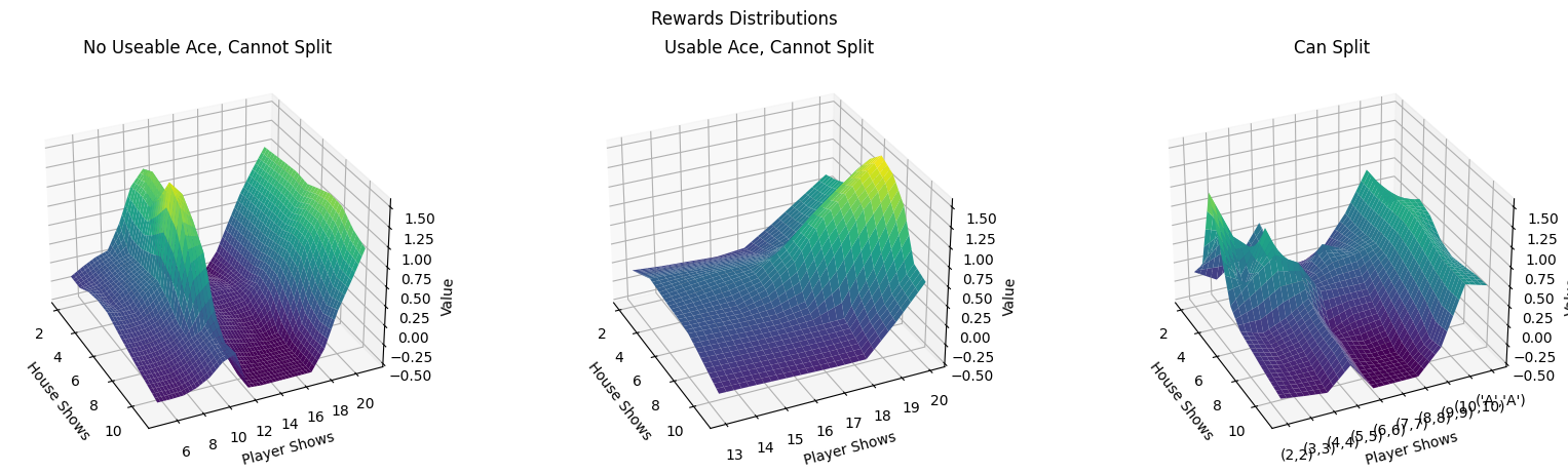
We achieve similar performance seen in my previous post, and the value functions seem quite similar.

By the end of gameplay, we can simulate 100 different games, where each game is played for 50 rounds. We on average achieve -0.0132 units of profit per hand.

Optimal Play

Similar to the logic behind generating the value function, I can explicitly list the optimal play according to the learned network. For each, if “double” was the optimal play, I also depict the next best alternative move if double was no longer available to us.

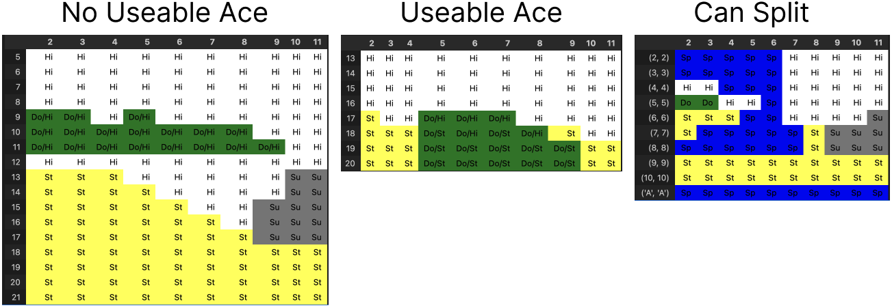
While there is a great amount of intuition behind “No useable ace” and likely “Can split”, the “Useable ace” category is not as intuitive. The “Can Split” seems to grossly underestimate the value of doubling on a pair of 5’s.

Conclusion

While blackjack, WITHOUT card count, is a tractable solution in the standard reinforcement learning framework, I provide a basic overview of how to adapt it to the deep q learning framework. I show the value functions and optimal gameplay based off this learned strategy. Admittedly, I don’t place a terribly big emphasis on optimizing the model and achieving high performance, however, results are sufficient for evaluating some baseline performance. By end of training, the model was able to achieve -0.0132 units won per round. This framework will be incredibly important for incorporating card count, which I’ll dive into much further in my next blog post!

Github is linked below :)