The goal of Curve V2 is to swap non-pegged token with a lower price impact than Uniswap (V2 and V3) while having the same divergent loss.

Curve V2 has been around for 2 years now and few people truly understand the specific features of Curve V2. So I’ll try to explain it in simple terms. Don’t hesitate to leave a comment if you don’t agree with what I write or if it isn’t clearly explained.

The explanation is divided into two articles :

• the bonding curve (Part I) [this article]

• the repegging algorithm (Part II) [to be published soon]

TL;DR

• Curve V2 changes the way we look at the bonding curve. In a classic bonding curve like a Constant Product Market Maker (xy=k), x and y refer to the balances of token x and y in the pool. Now, in Curve V2, x and y refer to the value of x and y in the pool (value=balance*price). This allows the equilibrium point to be in the “middle” of the bonding curve, just like it was with the swap of stablecoins in Curve V1.

• Thanks to a repegging algorithm which is run after each swap (and after an LP deposits or recovers liquidity), Curve V2 allows the swaps to occur near the equilibrium point.

• There are 2 constants in Curve V2 (A and γ). Like in StableSwap (Curve V1), the variable A allows to define the flat region around the equilibrium point which gives very low price impact. The purpose of the new variable γ is to make the curve behave more like a CPMM as we move away from equilibrium. Indeed, we want low price impact but not that much because we are dealing with volatile assets (not pegged assets like in StableSwap).

• All this means that liquidity is automatically and dynamically shifted towards the equilibrium point. The degree of liquidity concentration is defined by A and γ.

Defining some variables to understand the curve

Some of the equations in the Curve V2 whitepaper have errors. Also to make things easier to understand, I sometimes rename certain variables (but I specify when this is the case).

To simplify everything, we will work with pools of only 2 tokens (x and y). Let’s imagine that we are working on the USDT/ETH pool. So we have x which is USDT and y which is ETH. It is therefore a simplified version of the tricrypto2 (USDT/WBTC/ETH).

Let’s define some variables :

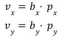
• bₓ : balance of x in the pool (number of token x in the pool)

• pₓ : priceScale of x in the pool. It gives the value of a token relative to a reference token from the pool. Generally we choose a stablecoin as a reference if there is one in the pool (so for us, pₓ=1 and pᵧ=1600 because 1 ETH = 1600 USDT). The priceScale is not necessarily the price of the token at the time of the swap. For the moment, we could said that this is an indicator of the token price and it is modified by the internal balancing algorithm (the repegging algorithm).

• vₓ : value of x in the pool (b’ in the whitepaper). We have :

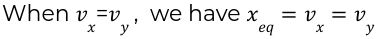
When we initialise the pool, the pool is at his equilibrium so :

The whitepaper introduces a variable xₑᵩ , the equilibrium point. xₑᵩ can be seen as the value of each token when we are at equilibrium (for example, when we initialise the pool) :

Now, let’s introduce D which is a dynamic value associated with the liquidity of the pool. At equilibrium, we have :

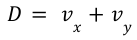
So :

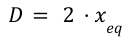
D does not have the same unit of measure as in Curve V1. Here D is expressed in value instead of balance like in V1.

A new approach of the bonding curve

The Constant Product Market Maker (CPMM) used in Uniswap is :

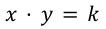
We can also write the CPMM with the variable D :

In a classic bonding curve like Uniswap or Curve V1, x and y refer to the balances of token x and y (bₓ and bᵧ). Now, the main idea of the Curve V2 whitepaper is to think of the bonding curve in terms of token value (vₓ and vᵧ), and no longer in terms of token balance (bₓ and bᵧ).

This completely changes the way we look at the bonding curve. This allows the equilibrium point to be in the middle of the Figure 1 (where vₓ=vᵧ). Thanks to this trick (and also the help of the reppeging algo), the swaps always occur in the “middle” of the bonding curve.

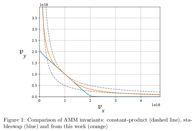
Michael Egorov could have used the CPMM function but CPMM is not optimised to reduce the price impact when we are around the equilibrium point. So to remedy this, Michael decided to take inspiration from his StableSwap curve.

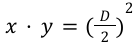
Let’s take a look at the StableSwap curve for a pool of 2 tokens :

If we divide by D, the StableSwap can also be seen as :

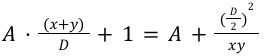
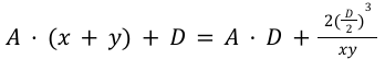
This curve is very flat around the equilibrium point which allows us to have very low price impact (indeed it is originally used to swap pegged assets). The greater the constant A, the flatter the curve. However for non-pegged assets we still want to have low price impact but not that much because we are dealing with volatile assets. Michael therefore introduced another variable called γ, and that’s how the V2 curve was born :

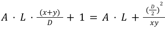
with

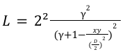
I have written this equation in this way (and not as in the whitepaper) in order to highlight the behaviour of the variable L. So let’s see :

The purpose of the variable γ is to make the curve behave more like a CPMM as you move away from equilibrium.

Indeed, when we move away from equilibrium :

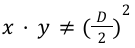
So :

So L will tends to :

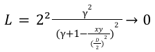
Meaning that the Curve V2 will tend to :

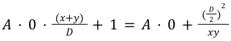
Which can be seen as :

Meaning that we have :

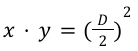
Wait…what?! It means that Curve V2 tends to a CPMM curve when we are moving away from the equilibrium point. Also, the lower the gamma value, the faster the curve behaves like a CPMM when moving away from equilibrium.

The same logic can be applied to show that the closer we get to equilibrium point (meaning xy → (D/2)²), the more L tends towards a constant and so the curve behaves like the StableCurve.

In a simplistic way, γ seems to be introduced to reduce the flat region inside the StableSwap curve. When gamma becomes smaller, the bounding curve becomes more like a constant product curve.

Now that we have cover the bonding curve and we have understand how Curve V2 allows low price impact, let’s focus on how Curve V2 is able to keep the swaps occur near the equilibrium point thanks to the repegging algorithm. Meaning how Curve V2 is able to move the center of liquidity to the equilibrium. [to be continued in the next article]

I’m Iñaki Cervera-Marzal, a senior data scientist who’s looking for a job in DeFi.

If you liked this article, feel free to mint it or share it. And if you want to support my work while having fun, you can mint one of my Nash suns NFT :)