Illia Dovhopolyi, Dmytro Zakharov

Linear operations, like those commonly used in neural networks, are very fast when calculated on a CPU. However, in ZK systems, they typically result in a large number of constraints, making them prohibitively expensive. In this article, we'll introduce a simple yet powerful optimization used in Bionetta that removes constraint costs for linear operations in R1CS circuits, making them absolutely free!

Linear Regression example

To illustrate this clearly, consider a simple linear regression circuit. We have two input vectors: x with length n, and w with length n+1. We want to constrain the following linear regression formula:

Here's how this circuit looks in Circom with n=100:

pragma circom 2.1.6;

template LinearRegression(n) {  
    signal input x[n];  
    signal input w[n+1];  
  
    signal output y;  
  
    signal t[n+1];  
    t[0] <== w[0];  
  
    for (var i = 0; i < n; i++) {  
        t[i+1] <== t[i] + x[i] * w[i+1];  
    }  
  
    y <== t[n];  
}

component main = LinearRegression(100);

Next, we compile this circuit into its R1CS representation:

circom circuits/LinearRegression.circom --r1cs --O1 -o artifacts

We can use the following JS script to count the number of R1CS and Plonk constraints generated by the circuit:

const snarkjs = require("snarkjs");  
const path = require("path");  
  
async function main() {  
    const ptauFile = path.join("artifacts", "powersOfTau28_hez_final_20.ptau");  
    const r1csFile = path.join("artifacts", "LinearRegression.r1cs");  
  
    const r1cs = await snarkjs.r1cs.exportJson(r1csFile);  
  
    console.log(`R1CS constraints: ${r1cs.nConstraints}`);  
  
    const zkeyFile = { type: "mem" };  
    await snarkjs.plonk.setup(r1csFile, ptauFile, zkeyFile, console);  
}
  
main().catch((e) => console.error(e));

Running this script gives us the following results:

> node index.js
R1CS constraints: 100
Plonk constraints: 201

This outcome isn't surprising. R1CS only counts constraints for multiplications, resulting in 100 constraints. In contrast, Plonk counts gates for both additions and multiplications, resulting in 201 constraints. We'll discuss these differences in more detail later.

Circuit embedded weights

So the previous approach becomes very expensive when we add many linear operations to our model. To optimize, we notice two important things:

1. Bionetta is a client-side proving framework, so we don't need to hide the model weights.

2. Weights only change when we retrain the model, not for each individual proof.

These points suggest embedding weights directly into the circuit as constants, rather than always passing them as signals.

You might wonder: what happens when the model is retrained, and the weights change? Won’t that invalidate the circuit? Indeed, it does — but our assumption here is that developers can simply recompile the circuit with the new weights and upgrade the verifier (usually on-chain contract). Although this adds certain inconveniences, we believe that it's a reasonable trade-off because it significantly reduces proving time for users.

Here's how this optimization looks in Circom, with weights set as constants. Here, we set w[i] = i for demonstration purposes. In practice, we'd use code generation to insert the actual trained weights:

pragma circom 2.1.6;  
  
template ConstantLinearRegression(n) { 
		// Below, we set compile-time known weights. In the actual 
		// Bionetta protocol, these values correspond to the real
		// trained values 
    var w[n+1];  
    for (var i = 0; i <= n; i++) {  
        w[i] = i;  
    }  
	  
	  // The rest is essentially the same, but the weights are known
    signal input x[n];
    signal output y;  
  
    var t = w[0];  
  
    for (var i = 0; i < n; i++) {  
        t += x[i] * w[i+1];  
    }  
  
    y <== t;  
}  
  
component main = ConstantLinearRegression(100);

Let's check how many constraints we now have using the same script as before:

> node index.js
R1CS constraints: 1
Plonk constraints: 100

Notice the huge improvement:

• R1CS linear operations became completely free - now we only have one constraint.

• All multiplication gates in Plonk disappeared, leaving us with only addition gates.

Why This Works

Let's first quickly recap how R1CS and Plonk arithmetizations work. Assume we have a witness: $\boldsymbol{z} = (1, z_1, z_2, \dots, z_{m-1})$.

In R1CS, the circuit is encoded by three matrices — $\mathbf{L}$, $\mathbf{R}$, and $\mathbf{O}$ — each of size $n \times m$ (where $n$ is the number of constraints and $m$ is the witness length). For the witness to be valid, we need to ensure that the following system of equations $\textbf{L}\boldsymbol{z} \circ \textbf{R}\boldsymbol{z} = \textbf{O}\boldsymbol{z}$ holds.

In Plonk, each constraint (or "gate") involves some specific witness elements $(l,r,o)$ (left, right, and output elements). Each gate also has five selectors $(q_M, q_L, q_R, q_O, q_C)$. These selectors are constant — analogous to the rows in the R1CS matrices — that define the gate's specific operation. For each gate, the following equation must hold:

Weights are signals

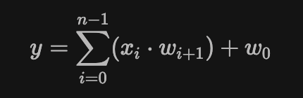
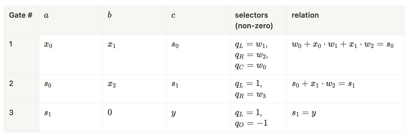
Suppose we have a small linear regression with three inputs $(x_0, x_1, x_2)$ and four weights $(w_0, w_1, w_2, w_3)$, computing:

We introduce intermediate accumulator elements:

And the output element:

Our full witness vector is:

It’s easy to show that enforcing this computation requires 3 R1CS constraints (or $n$ constraints for $n$ inputs):

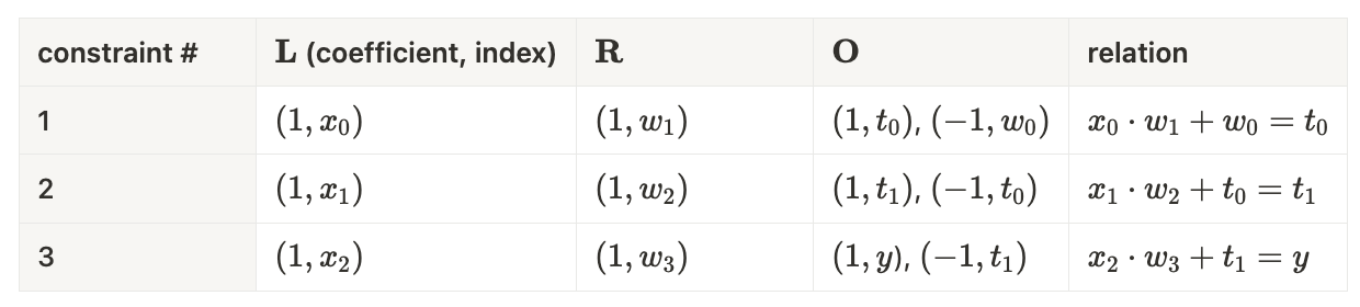
Constraints: $n$.

💡 Note: The first constraint includes the addition of a signal $w_0$. This is made possible by Gauss elimination, which Circom compiler performs automatically to simplify linear constraints.

In Plonk we need a dedicated gate for each addition, so we introduce extra intermediate values:

And we add a final copy constraint to expose the public output:

Putting everything together, the linear‑regression circuit with $n=3$ inputs requires 7 Plonk gates (in general, $2n+1$ gates):

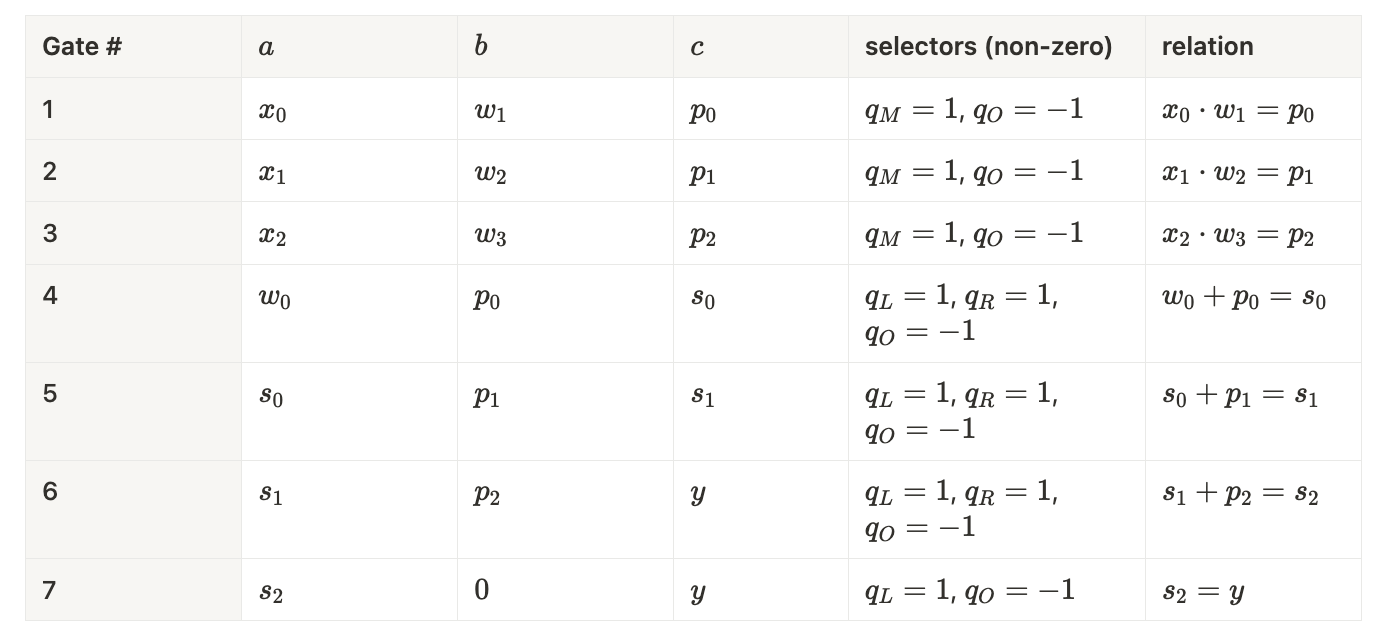
Gates: $2n+1$.

Weights are constants

Suppose we embedded the weights directly into the circuit. The same linear‑regression equation now reads:

Because the weights are no longer part of the witness, we can represent it as:

The beauty of this approach is that it collapses the entire computation into a single R1CS row: the constants $(w_0, w_1, w_2, w_3)$ now live in $\mathbf{L}$:

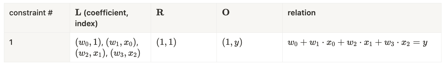
Constraints: 1.

In Plonk we can eliminate all multiplication gates by plugging the weights into the selectors, but each addition still needs its own gate. For $n=3$ inputs the circuit uses 3 gates (or $n$ gates in general):

Gates: $n$.

Benchmarks

To benchmark this optimization, we implemented a special MultiLinearRegression circuit and measured proving times for two scenarios: one with weights as signals, and the other with weights embedded as constants.

Here's how this circuit looks in Circom:

pragma circom 2.1.6;  
  
template ConstantMultiLinearRegression(n) {  
    var w[n][n+1];  
    for (var i = 0; i < n; i++) {  
        for (var j = 0; j <= n; j++) {  
            w[i][j] = i * n + j;  
        }  
    }  
    signal input x[n];  
  
    signal output out[n];  
  
    for (var i = 0; i < n; i++) {  
        var t = w[i][0];  
  
        for (var j = 0; j < n; j++) {  
            t += w[i][j+1] * x[j];  
        }  
  
        out[i] <== t;  
    }  
}  
  
component main = ConstantMultiLinearRegression(100);

And here's the equivalent implementation in Noir:

global W: [[Field; 101]; 100] = [...]

mod consts;  
  
fn const_multi_linear_regression<let N: u32>(x: [Field; N]) -> [Field; N] {  
    let mut out = [0; N];  
  
    for i in 0..N {  
        let mut t = consts::W[i][0];  
  
        for j in 0..N {  
            t += consts::W[i][j+1] * x[j];  
        }  
  
        out[i] = t;  
    }  
  
    out  
}

fn main(x: [Field; 100]) -> pub [Field; 100] {  
    const_multi_linear_regression::<100>(x)  
}

We recorded proving times across SnarkJS, RapidSnark, and Aztec Barretenberg implementations:

As demonstrated, embedding weights as constants significantly improves proving times for both R1CS and Plonk systems. R1CS systems are notably faster due to the substantial reduction in constraints. Interestingly, increasing the parameter n (representing the size of the linear regression) from 100 to 500 has minimal impact on proving times in R1CS-based proving systems.

Conclusion

In R1CS circuits, embedding the weights directly into the circuit makes linear operations completely free. This was one of the main reasons we chose to support R1CS‑based proving systems first in our client‑side proving framework, Bionetta. Together with our forthcoming optimization for non‑linear operations (see the next post on UltraGroth), this makes Bionetta exceptionally efficient: even large neural‑network models — such as a zkLiveness model — fit into roughly 100K constraints and can be proven very quickly.