Let’s be real—there’s nothing worse than gridding through a long-ass article only to realize you’ve spent 20 minutes getting to the good part. So, here’s the deal: before we dive in, we’re giving you the why. Why are multilinear extensions a big deal in the world of ZKPs? Because trust me, they are.

This article cuts through the noise and gives you everything you need to understand them—without endlessly searching the internet or looping through videos (like I did).

I’ve got you covered. Ready? Let’s jump right in!

Overview

First of all, don’t be worried if you’re not familiar with Sumcheck Protocol and GKR Protocol, we’ll cover them in other article. You only need to understand that we have a Prover and a Verifier. The Prover generates a proof $\pi$ using public and private inputs and sends it to the verifier that will later accept or reject.

1. Multilinear Extensions (MLEs):

   A function $f$ (with multiple inputs) can be transformed into a multilinear polynomial. This allows us to represent the function in a more "manageable" form for certain cryptographic protocols. In ZKP systems, this is essential because polynomials have nice properties (like interpolation), which help in proving things efficiently. By turning a function into a polynomial, the prover can later prove things about it (like evaluations) without revealing the whole function.

2. Sumcheck Protocol:

   This is a way to prove that a sum over a large number of values (typically from a multilinear polynomial) is correct. Imagine you want to prove that the sum of evaluations of your multilinear polynomial at many points equals some value. Instead of having the verifier check every single evaluation (which is costly), the prover can use the sumcheck protocol to prove it with only a few rounds of interaction.

3. GKR Protocol (Goldwasser-Kalai-Rothblum):

   The GKR protocol is designed to verify computations over layered arithmetic circuits. These circuits consist of multiple layers of gates, each computing simple arithmetic functions like addition or multiplication. The protocol is structured to efficiently verify computations on these circuits. It allows a verifier to check the correctness of a computation (like a circuit or a function evaluation) by checking only a few random positions in the multilinear extension of the function.

   In your case, after the prover creates the multilinear extension and runs the sumcheck protocol, the GKR protocol can be used to verify that the entire computation (represented by the circuit) was done correctly using MLEs and sumcheck. The GKR protocol verifies whether the result of the computation is correct without requiring the verifier to redo the entire computation.

How They Work Together

• The prover takes a function (or computation) and transforms it into a multilinear extension (using MLE).

• The sumcheck protocol helps prove that the sum of evaluations of this multilinear polynomial is correct.

• The GKR protocol adds an extra layer by allowing the verifier to check that this computation was done correctly with minimal effort.

The process becomes non-interactive by applying Fiat-Shamir, allowing the prover to send the proof directly to the verifier, who can then easily check the proof without additional communication rounds.

What is an Extension ?

Imagine you have a function that works only on a specific set of values. For example, let's say you have a simple function that works on integers:

• For $x=1$, it gives 5

• For $x=2$, it gives 8

• For $x=3$, it gives 10

This function is only defined for $x=1,2,3$, but you might want to “extend” it so it works on other numbers like $x=1.5, \space x=2.7$, etc. That's called an extension—taking a function that works on a small set and extending it to work on more values.

Multilinear Extensions

Now, instead of just having one variable (like $x$), imagine you have multiple variables (like $x$ and $y$). A multilinear extension is when you take a function that only gives you results at specific combinations of values (like a list or table of results) and extend it to fill in all the gaps between those values. This means the function will work not just at those specific points but smoothly across all values in between.

Original Function (Specific Points Only)

Let's say we have a function that gives values only at specific points for $x$ and $y$. For example:

In this table, the function is only defined for $x=0$ or $1$, and $y=0$ or $1$.

But this function does not tell us what happens when $x = 0.5$ or $y = 0.5$, or other values in between.

Multilinear Extension (Filling in the Gaps)

Now, the multilinear extension smoothly fills in the gaps between the known points. It creates new values for points like $x=0.5, \space y=0.5$, etc. The table might look something like this:

Now, the function provides values not just for $x=0$ and 1, but also for points in between, like $x=0.5$, $y=0.5$. The values are calculated in a way that ensures smooth changes between the known points.

So, the multilinear extension allows the function to work not just at the original grid points (like $x=0$, $y=0$) but also at every point in between, like $x=0.5$, $y=0.5$, while ensuring the transitions are smooth and linear.

Why use it in ZKPs ?

In protocols like GKR, you're often working with huge amounts of data, but you want to prove things efficiently. Instead of dealing with all the data points individually, you can summarize the behavior of a function over a small set of values and then extend it to cover the whole space. This makes the computation easier and faster while preserving the structure of the data.

The Core Idea

The key idea is that multilinear extensions allow you to deal with complex, multi-variable functions in a more efficient way, by extending them from a small number of points to a larger range, while still keeping the math manageable.

Visualization

Imagine you're looking at a huge high-resolution picture (like 4K). Instead of sending or analyzing every single pixel, you take a few key points that define the overall image (like the corners and a few central spots). Then, you use these points to reconstruct the image at a lower resolution. It saves time, but you still get a good idea of what the whole picture looks like.

This is similar to how multilinear extensions work in ZKPs: you only work with a few key data points, extend the function over the rest of the space, and still have enough information to prove things about the whole dataset.

Example

If you have a dataset of 10 elements, you can pick 2 or 3 key elements, use those to create a multilinear extension of the function, and then evaluate that function on 4 or 5 elements to get a good representation of how the function behaves across the entire set. This way, you avoid the need to process all 10 elements directly.

Small Exercise

Let's do a simple exercise for a multilinear extension using two variables $x$ and $y$. I’ll explain the step-by-step process and then walk you through the solution.

Given the following values for a function $f(x,y)$ at four points:

Goal : Construct the multilinear extension of $f(x,y)$, and find the value of the function at $(0.5,0.5)$.

Steps

1. Start with the four known Key Points. We know the values of the function at $(0,0), (0,1), (1,0)$ and $(1,1)$.

2. Define the multilinear extension formula. For two variables, the multilinear extension is a bilinear interpolation between the known points.

   Bilinear Interpolation: is a fixed formula that applies universally when you have values at the four corners of a grid (in two dimensions) and by four corners I mean the four Key points $(0,0), (0,1), (1,0) (1,1)$. It always follows the same structure because it's derived from linear interpolation along two axes. (You can watch a video on Youtube that explains this formula in depth if want to know how its built).

   The general formula is :

   $$f(x,y)= \textcolor{skyblue}{f(0,0)}⋅(1−x)(1−y)+\textcolor{skyblue}{f(1,0)}⋅x(1−y)+\textcolor{skyblue}{f(0,1)}⋅(1−x)y+\textcolor{skyblue}{f(1,1)}⋅xy$$

3. Substitute the known values of the function into the formula :

   $$f(x,y)=\textcolor{skyblue}{1}⋅(1−x)(1−y)+\textcolor{skyblue}5⋅x(1−y)+\textcolor{skyblue}3⋅(1−x)y+\textcolor{skyblue}7⋅xy$$

4. Find the value at $(0.5,0.5)$ by plugging $x=0.5$ and $y=0.5$ into the formula:

   $$f(0.5,0.5)=\textcolor{skyblue}1⋅(1−0.5)(1−0.5)+\textcolor{skyblue}5⋅0.5(1−0.5)+\textcolor{skyblue}3⋅(1−0.5)⋅0.5+\textcolor{skyblue}7⋅(0.50⋅0.5)$$

5. Now let’s calculate that step by step:

   $$f(0.5,0.5)=\textcolor{skyblue}1⋅(0.5)(0.5)+\textcolor{skyblue}5⋅0.5(0.5)+\textcolor{skyblue}3⋅(0.5)(0.5)+\textcolor{skyblue}7⋅(0.5)(0.5)$$
   $$f(0.5,0.5)=\textcolor{skyblue}1⋅0.25+\textcolor{skyblue}5⋅0.25+\textcolor{skyblue}3⋅0.25+7⋅0.25$$
   $$f(0.5,0.5)=0.25+1.25+0.75+1.75=4$$

   Answer : The value of the multilinear extension of the function at $(0.5,0.5)$ is 4.

   This process shows how you can extend a function defined at a few specific points (in this case, 4 points) to other values (like $x=0.5, y=0.5$) using multilinear interpolation.

Notes

• A polynomial is considered multilinear if he has degree at most 1 in each variable for example: $(1-x_1)(1-x_2)$.

• $x^2_1x_2$ is not a multilinear polynomial because it has a variable with degree 2.

• Any function $f$ who’s domain is $\{ 0,1 \}^l$ has many extension polynomials but only one of them will be exactly multilinear of degree at most 1 in each variable.

Recap with some visualize

Here we have a function $f$ defined on two bit inputs $\{ 0,1 \}^2$.

$f$ has four inputs $(0,0), (0,1), (1,0)$ and $(1,1)$.

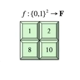
So for each of these four inputs, it spits out some field element:

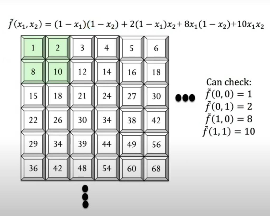
and here is its multilinear extension:

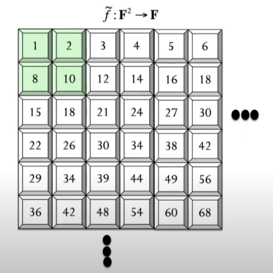
The multilinear extension polynomial is defined over all pairs of field elements. Often when we run these interactive proofs the field size is say $2^{64}$ or $2^{128}$.

If $f$ has these four inputs $(0,0), (0,1), (1,0), (1,1)$, we can express $\tilde{f}$ via Lagrange interpolation where sum each of the four inputs to $f$ and ensure that the polynomial your defining $\tilde{f}$ has exactly the current behavior on that input.

Lagrange interpolation and bilinear interpolation are both methods used for estimating unknown values, but they serve different purposes and are applied in distinct contexts. So this function is the same as the previous one we saw in the small exercise.

So for example if $f(0,0) = 1$, this function is the Lagrange basis polynomial that captures that.

So a function $f$ that has $\{ 0,1 \}^l$ or $2^l$ inputs will take $O(2^l)$-time (linear time) algorithm for evaluating $\tilde{f}(r)$, $r$ being random points $(x_i,x_j)$ in the finite field $F^l$.

That concludes everything you need to know about Multilinear Extensions. It wasn't so hard, was it ? In the next article we’ll be covering a full guide on the sumcheck Protocol. If you think this article was helpful feel free to subscribe and share it, byby.